Comprehensive Financial Analysis Report: Stock Market Returns and Risk

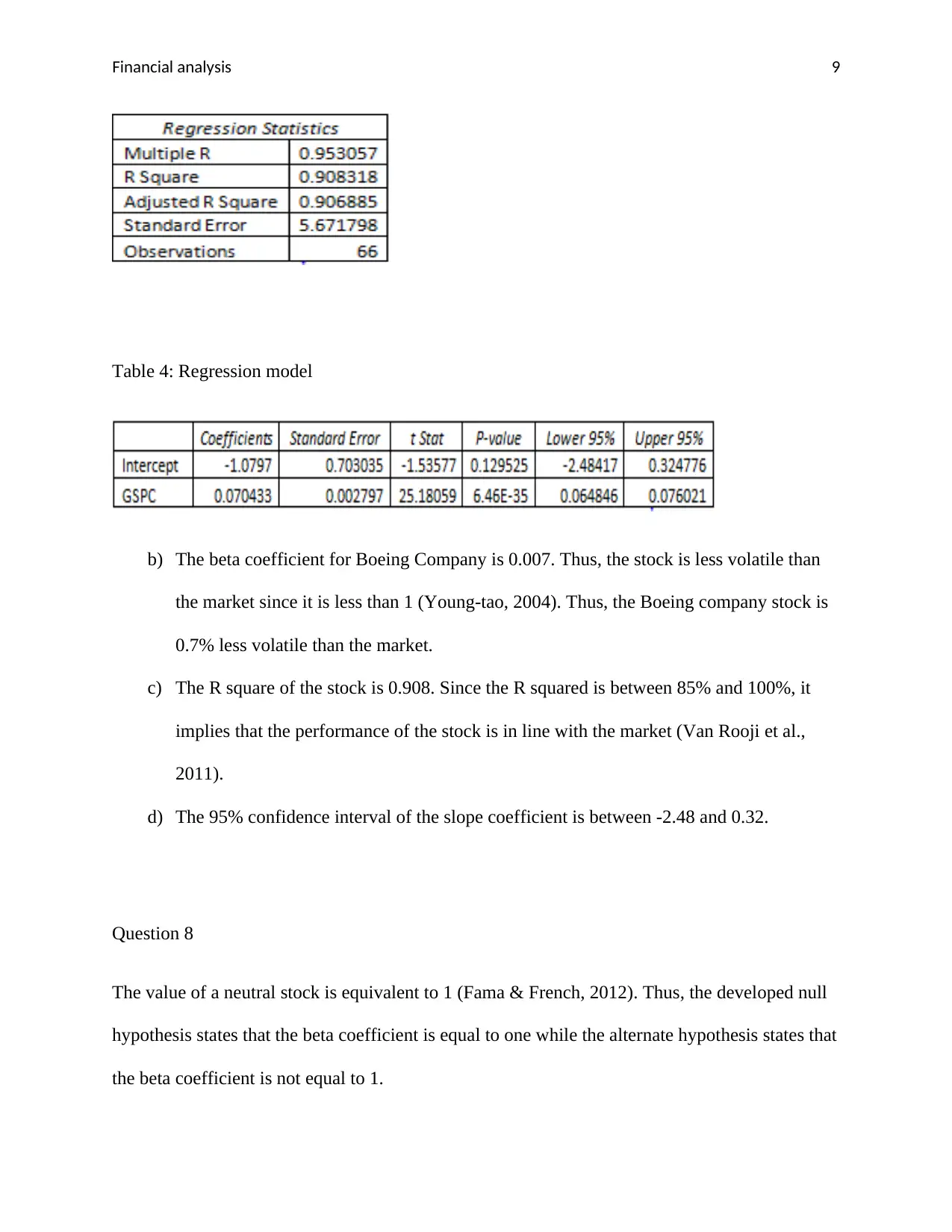
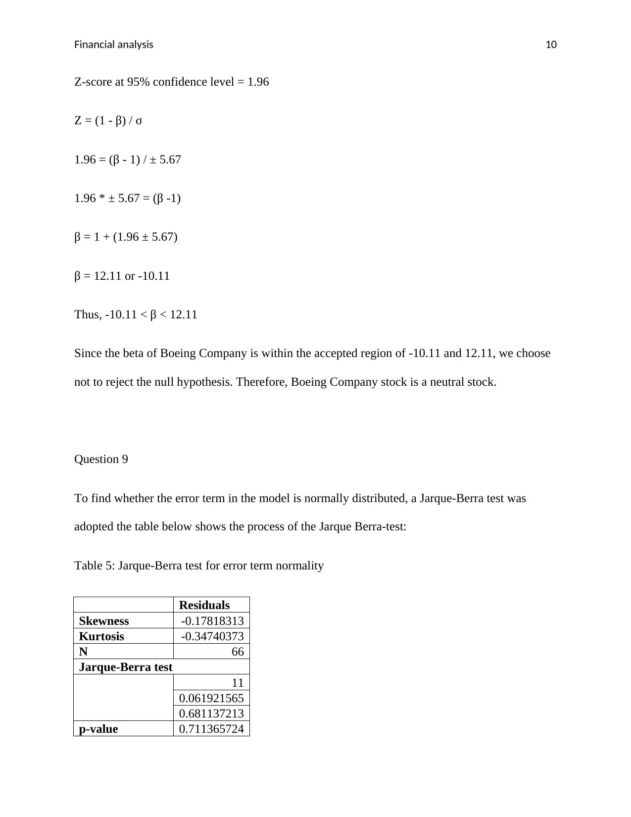
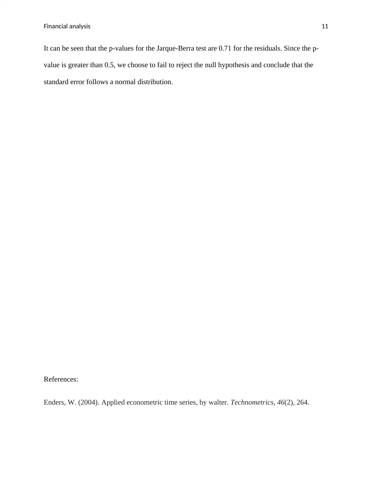
This report presents a comprehensive financial analysis of stock market data, focusing on the S&P 500, Boeing (BA), and IBM. The analysis begins with time series charts to visualize trends, cycles, and outliers in stock prices. Statistical methods are employed to calculate and compare returns, standard deviations, and risks associated with each stock. Hypothesis testing, including the Jarque-Bera test for normality, one-tailed z-tests, chi-square tests, and ANOVA, are used to evaluate stock performance and relationships between variables. The report further delves into regression analysis to determine beta coefficients and assess the volatility of Boeing stock relative to the market. The findings include insights into stock returns, risk assessment, and statistical validation of the results, concluding with a discussion of the preferred stock based on the analysis and the evaluation of the error term normality.

Running Header: FINANCIAL ANALYSIS 1
Financial Analysis
Student's name:
Institution:
Professor's name:
Course:

Financial analysis 2
Question 1
Line charts are used to display information as a data point series that are connected by straight
line segments (Kumar & Phrommathed, 2005). Line charts can be used to depict the features of
time series, thereby, there are referred to as time series graphs when the component of time is
included. As a result, time series carts are vital in determining the patterns of a model over a
period of time (Enders, 2007). The time series charts to be developed for S&P 500, BA and IBM
are needed to describe vital features of the time series pattern, to forecast future series' values,
explain how the past impacts the future, and to maybe provide a controlled standard for a
variable. The vital characteristics considered in a time series include the trend, long-run cycle,
seasonality, outliers, constant variance and abrupt changes (Shumway & Stoffer, 2006).
a) S&P 500 Price
Figure 1: S&P 500 price time series
7/1/2010
1/1/2011
7/1/2011
1/1/2012
7/1/2012
1/1/2013
7/1/2013
1/1/2014
7/1/2014
1/1/2015
7/1/2015
0
500
1000
1500
2000
2500
PS&P

Financial analysis 3
From figure 1 it can be seen that the S&P 500 has a trend which is increasing over time. The
trend can be observed by the straight line connecting the start point and the end point. However,
the trend does not show any seasonality as there are no significant outliers. Other observations
that can be made from the time series are that the S&P 500 has no abrupt changes and no period
unrelated to seasonality factors.
b) Boeing Company (BA) Stock Price
Figure 2: BA stock price time series
7/1/2010
1/1/2011
7/1/2011
1/1/2012
7/1/2012
1/1/2013
7/1/2013
1/1/2014
7/1/2014
1/1/2015
7/1/2015
0
20
40
60
80
100
120
140
160
PB
Like the S&P time series, it can be seen that the trend for Boeing Company is increasing
over time. The figure shows that the trend line has outliers. The outliers are values which are far
away from the trend line. However, it can be seen that the time series has no abrupt changes, no
seasonality or any long-run-cycle.
c) International Business Machine (IBM) stock price
Figure 3: IBM stock price time series

Financial analysis 4
7/1/2010
1/1/2011
7/1/2011
1/1/2012
7/1/2012
1/1/2013
7/1/2013
1/1/2014
7/1/2014
1/1/2015
7/1/2015
0
50
100
150
200
250
PIB
From figure 3, it is seen that IBM has no trend. Thus, the price of stocks can be seen to
rise from 7/1/2010 to1/1/2013. From 1/1/2013, the prices of the stock have been on the decline.
Moreover, due to a lack of a trend, the stocks can be seen to have no seasonality (Koopman &
Lee, 2009). Thus, there are no regular repeating patterns of high and lows. Conversely, the time
series has no abrupt changes, outliers, and long-run cycle.
Question 2
a) Calculated return for the three-time series can be observed in the Excel document.
b) The summarized statistics for the return series of the sample are shown in the diagram
below:
Table 1: Returns summary statistics
Summary statistics
S&P BA IBM
Average 0.950947
1.15744
3 0.106686
Variance 12.37148 33.3197 22.12779

Financial analysis 5
4
Standard deviation 3.517311
5.77232
5 4.704019
Table 1 shows that Boeing Company (1.157) has the highest return compared to IBM
(0.107). Moreover, Boeing Company has the highest standard deviation (5.77) compared to IBM
(4.7). It should be noted that the standard deviation of a stock measures its risk (Pastor & Robert,
2003). In addition, when the standard deviation is high, it shows that the stock is riskier. Thus,
Boeing Company is riskier than IBM even though the returns are higher. As a result, it can be
concluded that the average return of a stock has a linear relationship with the risk (Whitelaw,
2000). The S&P has an average return of 0.95 with a standard deviation of 3.5. Thus, the low
standard deviation of the index shows that the market returns are less volatile. On the other hand,
the average returns are relatively high as they are recorded at 0.95.
c) The Jarque-Berra test of return normality is shown in the workings below. The first step
involved the development of a hypothesis. The null hypothesis states that the returns of
Boeing Company stock and IBM stock are normally distributed. Alternatively, the
alternate hypothesis states that the returns of Boeing Company stock and IBM are not
normally distributed.
Table 2: Jarque-Berra of return normality test derivation
BA IBM
Skewness -0.18027 -0.40065
Kurtosis -0.40983 0.304225
N 65 65
Jarque-Berra test statistics
0.80693
6 1.989663
p-value 0.669 0.370
From table 2, it can be seen that the p-values for the Jarque-Berra test are 0.67 for Boeing
Company and 0.37 for IBM. Since the p-value is greater than 0.5, we choose to fail to not accept

Financial analysis 6
the null hypothesis that the returns are normally distributed. Therefore, Boeing Company and
IBM returns are normally distributed. Normality tests are carried out in order to determine the
appropriate tests that should be applied to the data (Jarque, 2011).
Question 3
To test the hypothesis that the average return of Boeing Company is greater than 3%, we choose
to perform a one-tailed z-test. Moreover, the test opts to check one direction, which is greater
than 3% (Franz et al., 2009).
The null hypothesis developed states that the average return on Boeing company stock is at least
3% while the alternate hypothesis states that the average return on Boeing company stock is less
than 3%.
Based on the formula; Z = (x̅ - μ)/(σ/(√n)), the z tests statistics derived will be equal to 1.574.
The critical value for α = 0.05 for a one-tailed test is 1.645. Since 1.574 is less than 1.645, it is in
the acceptance region. Therefore, the average return of Boeing Company is at least 3%.
Question 4
To compare the risk associated to each of the two stocks, a chi-square test was adopted. The chi-
square test was adapted since it tests the relationship between categorical variables (Zibran,
2007).

Financial analysis 7
The null hypothesis developed states that the standard devotions of the two stocks are equal. On
the other hand, the alternate hypothesis states that the standard deviations of the two stocks are
not equal.
The α to be used for this test is equal to 0.05. On the other hand, the numerator degree of
freedom and the denominator degree of freedom are both 64 that is 65-1.
Thus, using the formula; F = σ2 1
σ2 2, the derived F test statistics is 1.506.
Critical values: F (0.975, 64, 64) = 0.54
F (0.025, 64, 64) =1.0
Rejection region: Reject H0 if F < 0.54 or F > 1.0
Thus, there is enough evidence to not accept the null hypothesis since the F statistic is within the
acceptance region. Therefore, the risks associated with the stock are similar to each other.
Question 5
To determine whether the population average returns are equal, an ANOVA analysis was chosen.
The results of the ANOVA analysis are shown below:
The null hypothesis developed states that the population average returns are equal while the
alternate hypothesis states that the population averages are not equal.
Table 3: Summary

Financial analysis 8
Groups Count Sum Average
Varianc
e
BA 65
61.8115
6
0.95094
7
12.3714
8
IBM 65
75.2337
7
1.15744
3
33.3197
4
Table 4: ANOVA
The P-value of the ANOVA test is greater than the significance level of 5%. Thus, the decision is
to reject the null hypothesis. Therefore, the population average returns of the two stocks are not
the same.
Question 6
Computation of excess returns as seen in the attached excel document.
Question 7
a) The preferred stock is Boeing Company
Table 5: Regression statistics

Financial analysis 9
Table 4: Regression model
b) The beta coefficient for Boeing Company is 0.007. Thus, the stock is less volatile than
the market since it is less than 1 (Young-tao, 2004). Thus, the Boeing company stock is
0.7% less volatile than the market.
c) The R square of the stock is 0.908. Since the R squared is between 85% and 100%, it
implies that the performance of the stock is in line with the market (Van Rooji et al.,
2011).
d) The 95% confidence interval of the slope coefficient is between -2.48 and 0.32.
Question 8
The value of a neutral stock is equivalent to 1 (Fama & French, 2012). Thus, the developed null
hypothesis states that the beta coefficient is equal to one while the alternate hypothesis states that
the beta coefficient is not equal to 1.

Financial analysis 10
Z-score at 95% confidence level = 1.96
Z = (1 - β) / σ
1.96 = (β - 1) / ± 5.67
1.96 * ± 5.67 = (β -1)
β = 1 + (1.96 ± 5.67)
β = 12.11 or -10.11
Thus, -10.11 < β < 12.11
Since the beta of Boeing Company is within the accepted region of -10.11 and 12.11, we choose
not to reject the null hypothesis. Therefore, Boeing Company stock is a neutral stock.
Question 9
To find whether the error term in the model is normally distributed, a Jarque-Berra test was
adopted the table below shows the process of the Jarque Berra-test:
Table 5: Jarque-Berra test for error term normality
Residuals
Skewness -0.17818313
Kurtosis -0.34740373
N 66
Jarque-Berra test
11
0.061921565
0.681137213
p-value 0.711365724

Financial analysis 11
It can be seen that the p-values for the Jarque-Berra test are 0.71 for the residuals. Since the p-
value is greater than 0.5, we choose to fail to reject the null hypothesis and conclude that the
standard error follows a normal distribution.
References:
Enders, W. (2004). Applied econometric time series, by walter. Technometrics, 46(2), 264.

Financial analysis 12
Fama, E. F., & French, K. R. (2012). Size, value, and momentum in international stock
returns. Journal of financial economics, 105(3), 457-472.
Faul, F., Erdfelder, E., Buchner, A., & Lang, A. G. (2009). Statistical power analyses using G*
Power 3.1: Tests for correlation and regression analyses. Behavior research
methods, 41(4), 1149-1160.
Koopman, S. J., & Lee, K. M. (2009). Seasonality with trend and cycle interactions in
unobserved components models. Journal of the Royal Statistical Society: Series C
(Applied Statistics), 58(4), 427-448.
Jarque, C. M. (2011). Jarque-Bera test. In International Encyclopedia of Statistical Science (pp.
701-702). Springer Berlin Heidelberg.
Kumar, S., & Phrommathed, P. (2005). Research methodology (pp. 43-50). Springer US.
Pástor, Ľ., & Stambaugh, R. F. (2003). Liquidity risk and expected stock returns. Journal of
Political economy, 111(3), 642-685.
Shumway, R. H., & Stoffer, D. S. (2006). Time series analysis and its applications: with R
examples. Springer Science & Business Media.
Van Rooij, M., Lusardi, A., & Alessie, R. (2011). Financial literacy and stock market
participation. Journal of Financial Economics, 101(2), 449-472.
Whitelaw, R. F. (2000). Stock market risk and return: An equilibrium approach. The Review of
Financial Studies, 13(3), 521-547.

Financial analysis 13
Yong-tao, L. I. U. (2004). An Empirical Study on Beta Coefficient and Its Related Characteristic
in Shanghai Stock Market [J]. Policy-making Reference, 1.
Zibran, M. F. (2007). Chi-squared test of independence. Department of Computer Science,
University of Calgary, Alberta, Canada.