Analyzing Investment Decisions with Decision Support Tools

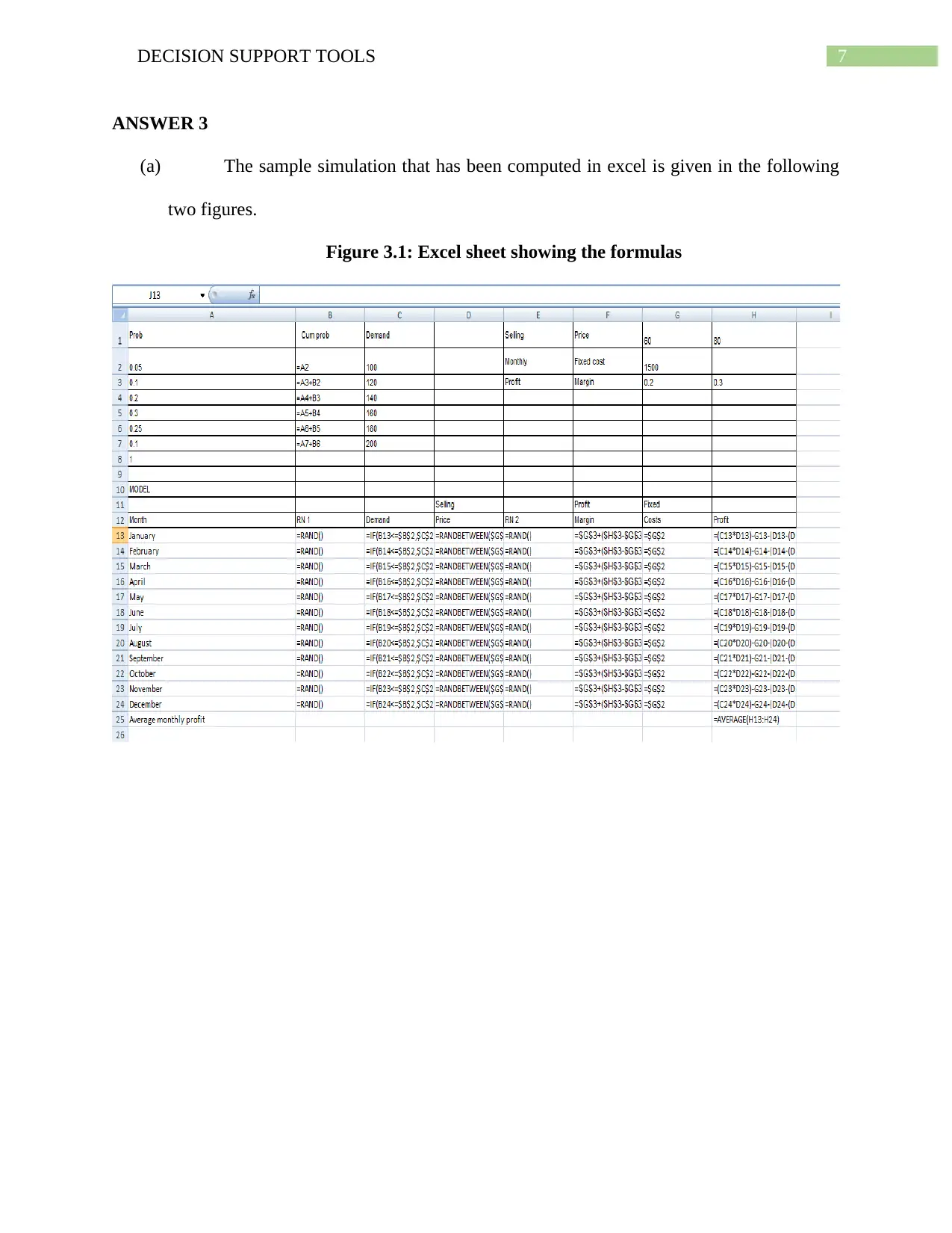
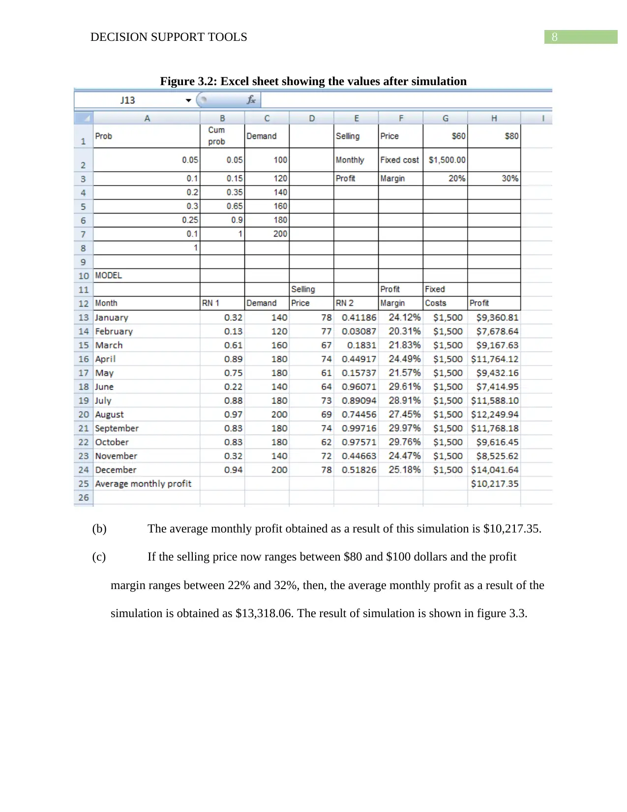
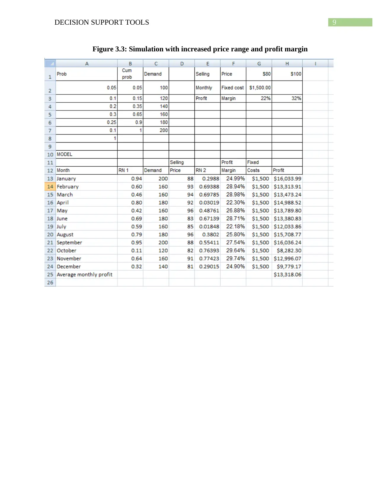
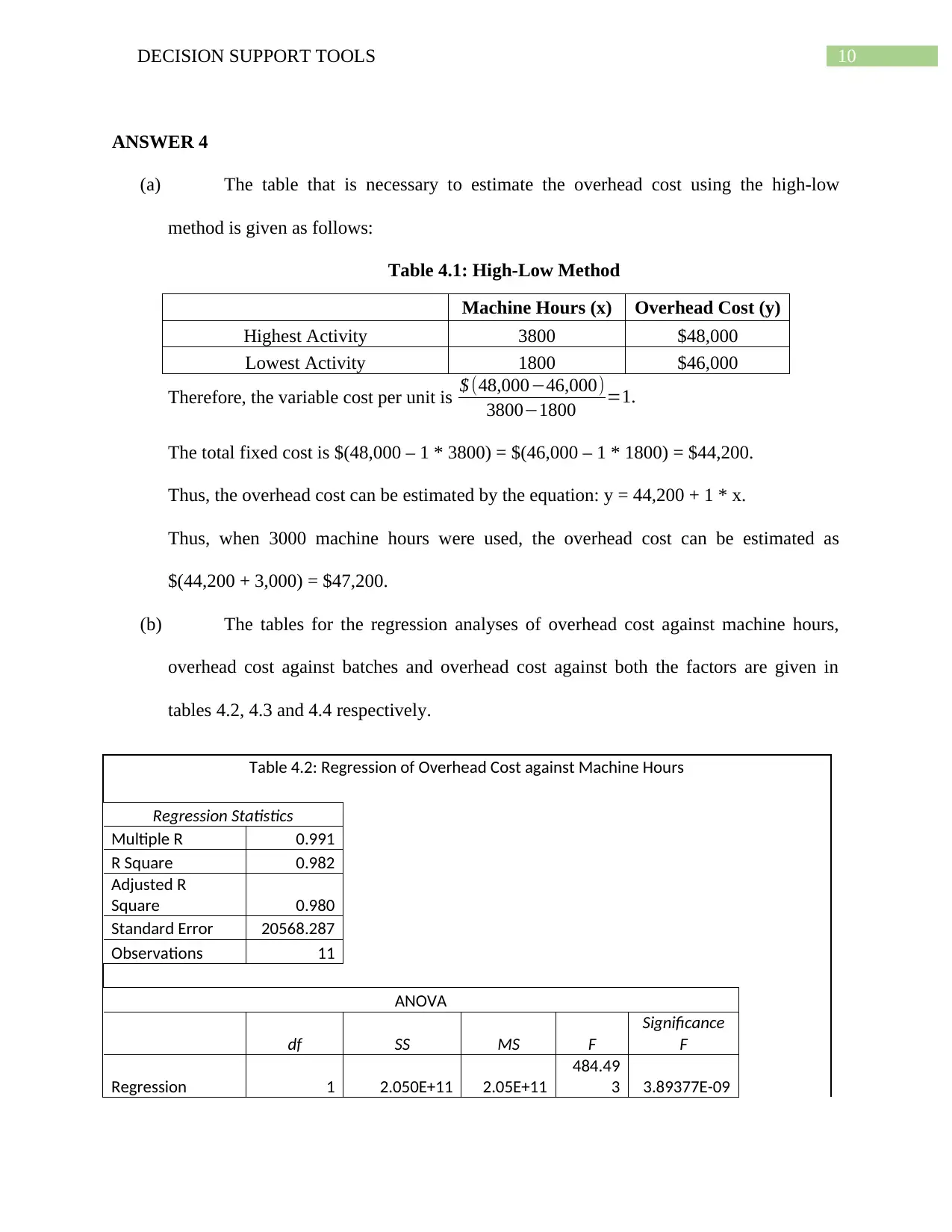
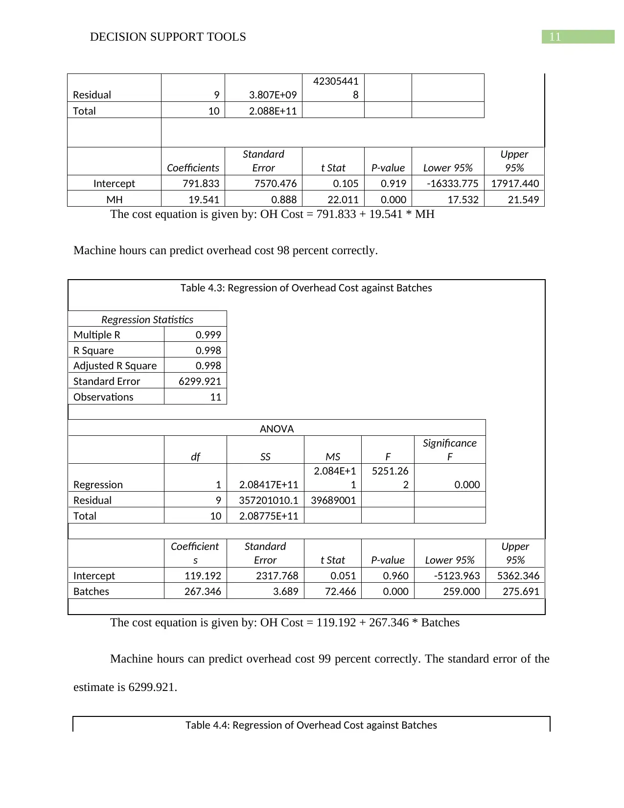
This assignment delves into the application of decision support tools in financial decision-making. It begins by differentiating between decision-making under certainty, risk, and uncertainty, using a payoff matrix to analyze investment options (share market, bonds, real estate) under different economic scenarios. The assignment explores the perspectives of optimists, pessimists, and the criterion of regret, along with expected value calculations and the expected value of perfect information (EVPI). Further, it examines a bicycle shop scenario, incorporating prior and posterior probabilities, and the value of market research. A simulation is performed using Excel to analyze average monthly profits under varying conditions. Additionally, the assignment employs the high-low method and regression analysis to estimate overhead costs, comparing the predictive power of machine hours and batches. Finally, it analyzes break-even points for two products and determines the sales volume needed to achieve target profits before and after tax, considering a product mix ratio.

Running Head: DECISION SUPPORT TOOLS
Decision Support Tools
Name of the Student
Name of the University
Author Note

1DECISION SUPPORT TOOLS
Table of Contents
ANSWER 1.....................................................................................................................................2
ANSWER 2.....................................................................................................................................4
ANSWER 3.....................................................................................................................................6
ANSWER 4.....................................................................................................................................7
ANSWER 5...................................................................................................................................10

2DECISION SUPPORT TOOLS
ANSWER 1
(a) Decision making under certainty describes a situation where a decision maker has
to make a decision when there are all the necessary information that are required to make
a decision present.
Decision making under risk describes a situation where all the decisions that can
be made has a particular probability of occurrence.
Decision making under uncertainty describes a situation where the decision maker
has to make a decision when there is incomplete or no information that are required to
make a decision.
(b) Bikram Shrestha inherited some money and he wants to invest it in share markets,
bonds, or real estates. The payoff matrix showing the profits of the markets for the next
year are given below:
Good Economy Poor Economy
Share market $80,000 ($20,000)
Bonds 30,000 20,000
Real estate 25,000 15,000
1. An optimist would choose the alternative in which the maximum payoff is
maximized. From the following table 1, it can be seen that the maximum profit
can be earned from share markets. Thus, the decision of an optimist would be to
invest in share markets.

3DECISION SUPPORT TOOLS
Table 1: Decision of an optimist
Good Economy Poor Economy Best
Share market $80,000 ($20,000) $80,000
Bonds $30,000 $20,000 $30,000
Real estate $25,000 $15,000 $25,000
2. A pessimist would choose the alternative in which the minimum payoff is
maximized. From the following table 2, it can be seen that the maximum profit
from the minimum payoffs can be earned from bonds. Thus, the decision of a
pessimist would be to invest in bonds.
Table 2: Decision of a Pessimist
Good Economy Poor Economy Worst
Share market $80,000 -$20,000.00 -$20,000.00
Bonds $30,000 $20,000.00 $20,000.00
Real estate $25,000 $15,000.00 $15,000.00
3. A criterion of regret is defined as minimizing the maximum regret. Here,
regret indicates opportunity loss. Thus, regret = best payoff – payoff received.
Then, the first table can be framed as follows in terms of regret. The minimum
regret value has been found in Share market. Thus, the decision should be to
invest in share markets.
Table 3: Regret Table
Good Economy Poor Economy Maximum
Share market $0 $40,000.00 $40,000.00
Bonds $50,000 $0.00 $50,000.00
Real estate $55,000 $5,000.00 $55,000.00
4. It has been assumed that the probability of a good economy is 0.3. Thus,
the probability of a poor economy is (1 – 0.3) = 0.7. Thus, the expected profits in
Share Market = (0.3 * $80,000) – (0.7 * $20,000) = $10,000.
Bonds = (0.3 * $30,000) + (0.7 * $20,000) = $23,000.
Real Estate = (0.3 * $25,000) – (0.7 * $15,000) = $18,000.

4DECISION SUPPORT TOOLS
Thus, the optimal action will be to invest in Bonds according to the
assumption in this question.
5. The expected value of perfect information (EVPI) is given by the formula
EVPI=∑
j
p j ( max
i Rij )−max
i ∑
j
p j Rij, where, Rij is the value of the ith row and jth
column and pj is the probability of that cell.
Thus, ∑
j
p j (max
i Rij ) = (0.3 * $80,000) + (0.3 * $30,000) + (0.3 * $25,000) =
$40,500.
Again, max
i ∑
j
p j Rij=¿$23,000.
Therefore, EVPI = $(40,500 – 23000) = $17,500.

5DECISION SUPPORT TOOLS
ANSWER 2
(a) Jerry wants to open a bicycle shop. He can open two types of shops – large shops
(a1) and small shops (a2). There are two types of markets – good market (s1) and poor
market (s2). According to his beliefs, in a large shop, there will be a profit of $80,000 in a
good market and a loss of $40,000 in a poor market. There is a 50 percent chance for the
market to be good or bad. Thus, in a large shop, the estimated profit will be:
P (a1) = $80,000 * P (s1) + $(- 40,000) * P (s2)
= $(80,000 * 0.5 – 40,000 * 0.5)
= $20,000.
In a small shop, jerry believes that there will be a profit of $30,000 in a good
market and a loss of $10,000 in a poor market.Thus, in a small shop, the estimated profit
will be:
P (a2) = $30,000 * P (s1) + $(- 10,000) * P (s2)
= $(30,000 * 0.5 – 10,000 * 0.5)
= $10,000.
Thus, whether the market is good or bad, profit is more in a large shop compared
to a small shop. Thus, Jerry should open a large shop.
(b) Considering the track record provided by Jerry’s friend, The prior probabilities
has been revised. Here a favorable market has been considered as F and an unfavorable
market has been considered as U. Irrespective of good or poor market conditions, in an
unfavorable market, there has been no profit or loss. Thus, in a large shop, the revised
prior probability will be:
P (a1) = P (s1) * P (F) + P (s2) * P (U)

6DECISION SUPPORT TOOLS
= 0.5 * 0.8 + 0.5 * 0.2
= 0.5.
Thus, in a small shop, the revised prior probability will be:
P (a2) = P (s1) * P (F) + P (s2) * P (U)
= 0.5 * 0.8 + 0.5 * 0.4
= 0.5.
(c) The posterior probability of a good market given that his friend has provided an
unfavorable market prediction is P (s1) * P (U) = 0.5 * 0.2 = 0.1.
(d) The expected net gain in a large market is
P (a1) = $80,000 * P (s1) * P (F) + $(- 40,000) * P (s2) * P (U)
= $(80,000 * 0.5 * 0.8 – 40,000 * 0.5 * 0.2)
= $24,000.
The expected gain in small market is
P (a2) = $30,000 * P (s1) * P (F) + $(- 10,000) * P (s2) * P (U)
= $(30,000 * 0.5 * 0.8 – 10,000 * 0.5 * 0.2)
= $10,000.
If his friend is engaged to conduct the market research, the profit in the large
market will become $(24,000 – 3,000) = $21,000 and in the small market will become
$(10,000 – 3,000) = $7,000.
Thus, if his friend is engaged, his profit in the large market will increase and his
profit in the small market will decrease. Thus, there is not much increase in the profits by
engaging his friend and conducting the market research. Hence, his friend should not be
involved.

7DECISION SUPPORT TOOLS
ANSWER 3
(a) The sample simulation that has been computed in excel is given in the following
two figures.
Figure 3.1: Excel sheet showing the formulas

8DECISION SUPPORT TOOLS
Figure 3.2: Excel sheet showing the values after simulation
(b) The average monthly profit obtained as a result of this simulation is $10,217.35.
(c) If the selling price now ranges between $80 and $100 dollars and the profit
margin ranges between 22% and 32%, then, the average monthly profit as a result of the
simulation is obtained as $13,318.06. The result of simulation is shown in figure 3.3.

9DECISION SUPPORT TOOLS
Figure 3.3: Simulation with increased price range and profit margin

10DECISION SUPPORT TOOLS
ANSWER 4
(a) The table that is necessary to estimate the overhead cost using the high-low
method is given as follows:
Table 4.1: High-Low Method
Machine Hours (x) Overhead Cost (y)
Highest Activity 3800 $48,000
Lowest Activity 1800 $46,000
Therefore, the variable cost per unit is $ (48,000−46,000)
3800−1800 =1.
The total fixed cost is $(48,000 – 1 * 3800) = $(46,000 – 1 * 1800) = $44,200.
Thus, the overhead cost can be estimated by the equation: y = 44,200 + 1 * x.
Thus, when 3000 machine hours were used, the overhead cost can be estimated as
$(44,200 + 3,000) = $47,200.
(b) The tables for the regression analyses of overhead cost against machine hours,
overhead cost against batches and overhead cost against both the factors are given in
tables 4.2, 4.3 and 4.4 respectively.
Table 4.2: Regression of Overhead Cost against Machine Hours
Regression Statistics
Multiple R 0.991
R Square 0.982
Adjusted R
Square 0.980
Standard Error 20568.287
Observations 11
ANOVA
df SS MS F
Significance
F
Regression 1 2.050E+11 2.05E+11
484.49
3 3.89377E-09

11DECISION SUPPORT TOOLS
Residual 9 3.807E+09
42305441
8
Total 10 2.088E+11
Coefficients
Standard
Error t Stat P-value Lower 95%
Upper
95%
Intercept 791.833 7570.476 0.105 0.919 -16333.775 17917.440
MH 19.541 0.888 22.011 0.000 17.532 21.549
The cost equation is given by: OH Cost = 791.833 + 19.541 * MH
Machine hours can predict overhead cost 98 percent correctly.
Table 4.3: Regression of Overhead Cost against Batches
Regression Statistics
Multiple R 0.999
R Square 0.998
Adjusted R Square 0.998
Standard Error 6299.921
Observations 11
ANOVA
df SS MS F
Significance
F
Regression 1 2.08417E+11
2.084E+1
1
5251.26
2 0.000
Residual 9 357201010.1 39689001
Total 10 2.08775E+11
Coefficient
s
Standard
Error t Stat P-value Lower 95%
Upper
95%
Intercept 119.192 2317.768 0.051 0.960 -5123.963 5362.346
Batches 267.346 3.689 72.466 0.000 259.000 275.691
The cost equation is given by: OH Cost = 119.192 + 267.346 * Batches
Machine hours can predict overhead cost 99 percent correctly. The standard error of the
estimate is 6299.921.
Table 4.4: Regression of Overhead Cost against Batches

12DECISION SUPPORT TOOLS
Regression Statistics
Multiple R 0.999
R Square 0.998
Adjusted R Square 0.998
Standard Error 6585.241
Observations 11
ANOVA
df SS MS F Significance F
Regression 2 2.08428E+11 1.042E+11 2403.156 7.62471E-12
Residual 8 346923227.2 43365403
Total 10 2.08775E+11
Coefficients Standard Error t Stat P-value Lower 95% Upper 95%
Intercept 66.444 2425.160 0.027 0.979 -5525.985 5658.872
MH 1.019 2.093 0.487 0.639 -3.807 5.845
Batches 253.650 28.394 8.933 0.000 188.173 319.128
The cost equation is given by: OH Cost = 66.444 + 1.019 * MH + 253.650 * Batches
Machine hours can predict overhead cost 99 percent correctly. The standard error of the
estimate is 6585.241.
(c) The standard error of the estimates was less when batches were used to predict the
overhead cost. Thus, the best regression will be considered batches in predicting
overhead cost. The variable explains 99 percent of overhead cost and has a lesser
standard error. Thus, batches are considered better predictor.
(d) Using the best regression result, OH Cost = 119.192 + 267.346 * Batches, the
projected overhead cost in a month in which there were 2000 machine hours worked and
150 batches produced is $(119.192 + 267.346 * 150) = $40221.09.

13DECISION SUPPORT TOOLS
ANSWER 5
(a) For product A, per unit sales price is $10 and per unit variable cost is $5. Thus,
the unit contribution of A is $(10 – 5) = $5.
(b) To reach the break-even point for product B, the manufacturer has to sell (4000/8)
= 500 units.
(c) To reach the break-even point for product A, the manufacturer has to sell (4000/5)
= 800 units.
(d) If the manufacturer decides to manufacture both product A and product B in the
ratio of 2:1 respectively, then
(i) To earn a profit of $5,000 before tax for the month,
Product A B Total
Sales Unit 2 1 2 + 1 = 3
Sales price 2 * $10 = $20 1 * $20 = $20 $20 + $20 = $40
Variable cost 2 * $5 = $10 1 * $12 = $12 $10 + $12 = $22
Total fixed costs $4,000
Total Contribution $20 - $10 = $10 $20 - $12 = $8 $10 + $8 = $18
Weighted average
Contribution $18 / 3 = $6
Targeted Profit (Before Tax) $5,000
Targeted Sales Volume (2/3) * 1500 =
1000
(1/3) * 1500 =
500
($4,000 + $5,000)/$6 =
1500
Thus, 1000 units of product A and 500 units of product B should be
manufactured to earn a profit of $5,000 before tax.
(ii) To earn a profit of $21,000 after tax for the month,
Product A B Total
Sales Unit 2 * $10 = $20 1 * $20 = $20 2 + 1 = 3
Sales price 2 * $5 = $10 1 * $12 = $12 $20 + $20 = $40
Variable cost $10 + $12 = $22
Total fixed costs $20 - $10 = $10 $20 - $12 = $8 $4,000
Total Contribution 2 * $10 = $20 1 * $20 = $20 $10 + $8 = $18
Weighted average $18 / 3 = $6

14DECISION SUPPORT TOOLS
Contribution
Targeted Profit (After Tax) $21,000
Tax Rate 30%
Targeted Profit (Before Tax) $21,000/(1 – 0.3) = $30,000
Targeted Sales Volume (2/3) * 5667 =
3778
(1/3) * 5667 =
1889
($4,000 + $21,000)/$6 =
5667
Thus, 3778 units of product A and 1889 units of product B should be
manufactured to earn a profit of $21,000 after tax.