Examining the 2007-09 Subprime Crisis: Causes & UK Regulatory Changes
VerifiedAdded on 2023/04/21
|15
|7862
|140
Essay
AI Summary
This essay examines the subprime crisis of 2007-2009, focusing on its micro and macro causes as well as the UK's subsequent financial regulation reforms. It begins by outlining the sequence of events in financial crises, highlighting the role of asymmetric information and the impact on financial markets. The analysis covers the global financial imbalances, low real interest rates, consumer inertia, corporate leverage, compensation schemes, and the role of rating agencies. It further details the stages of the crisis, from excessive lending in the US subprime market to the contagion throughout the global economy. The essay also addresses the UK governmental responses, including monetary, fiscal, and stabilization policies, and assesses their effectiveness in ameliorating the impact of the banking crisis. The assignment concludes by emphasizing the importance of understanding the factors that led to the crisis and the measures implemented by the Bank of England.

See discussions, stats, and author profiles for this publication at: https://www.researchgate.net/publication/289750481
Crisis periods and contagion effects in the CEE stock markets: the influence of
the 2007 US subprime crisis
Article · January 2016
DOI: 10.1504/IJCEE.2016.075612
CITATIONS
0
READS
53
2 authors:
Some of the authors of this publication are also working on these related projects:
Comparative research on commonality in liquidity on the Central and Eastern European stock markets (NCN, OPUS 11, 2016/21/B/HS4/02004)View project
BST/2017/2018View project
Joanna Olbrys
Bialystok University of Technology
86PUBLICATIONS307CITATIONS
SEE PROFILE
Elzbieta Majewska
University of Bialystok
24PUBLICATIONS96CITATIONS
SEE PROFILE
All content following this page was uploaded by Joanna Olbrys on 13 July 2016.
The user has requested enhancement of the downloaded file.
Paraphrase This Document
Need a fresh take? Get an instant paraphrase of this document with our AI Paraphraser
124 Int. J. Computational Economics and Econometrics, Vol. 6, No. 2, 2016
Copyright © 2016 Inderscience Enterprises Ltd.
Crisis periods and contagion effects in the CEE stock
markets: the influence of the 2007 US subprime crisis
Joanna Olbrys*
Faculty of Computer Science,
Bialystok University of Technology,
Wiejska 45A, 15–351 Bialystok, Poland
Email: j.olbrys@pb.edu.pl
*Corresponding author
Elzbieta Majewska
Faculty of Mathematics and Informatics,
University of Bialystok,
K. Ciolkowskiego 1M, 15-245 Bialystok, Poland
Email: elam@math.uwb.edu.pl
Abstract: The main goal of this paper is a direct identification of crisis periods
in the eight Central and Eastern European (CEE) equity markets, and, for
comparison, in the US market. A statistical procedure of dividing market
states into up and down markets is employed. The results confirm
October 2007–February 2009 as the common period of the recent global
financial crisis in the CEE markets, except for Slovakia. Moreover, the effect of
increasing cross-market correlations in the crisis period in the context of
contagion is investigated, applying both standard contemporaneous correlations
and volatility-adjusted correlation coefficients. A research hypothesis that there
was no contagion effect among the US and the CEE stock markets during the
2007–2009 crisis is explicitly tested. The robustness analysis of contagion tests
based on monthly, weekly and daily data is provided. The results reveal that the
utilised tests are rather less sensitive with respect to the choice of data
frequency.
Keywords: CEE stock markets; crisis period; market states; cross-market
correlations; contagion.
Reference to this paper should be made as follows: Olbrys, J. and
Majewska, E. (2016) ‘Crisis periods and contagion effects in the CEE stock
markets: the influence of the 2007 US subprime crisis’, Int. J. Computational
Economics and Econometrics, Vol. 6, No. 2, pp.124–137.
Biographical notes: Joanna Olbrys is an Assistant Professor at the Faculty of
Computer Science, Bialystok University of Technology. She holds her PhD in
Technical Sciences on Control Engineering and Robotics from the Systems
Research Institute of Polish Academy of Sciences in Warsaw. She was the
Head and the Principal Investigator of a research project financially supported
by the Polish Ministry of Science and Higher Education. She has a large
number of publications in various scientific journals such as Emerging Markets
Finance and Trade, Argumenta Oeconomica, Operations Research and
Decisions, La Pensée, Chinese Business Review, Folia Oeconomica Stetinensia
Crisis periods and contagion effects in the CEE stock markets 125
and Dynamic Econometric Models, Control and Cybernetics. She acts as a
Referee to Tourism Management, International Review of Economics and
Finance, Economic Modelling and Acta Oeconomica.
Elzbieta Majewska is an Assistant Professor at the Faculty of Mathematics
and Informatics, University of Bialystok. She holds her PhD in Economics
from the Warsaw University of Life Science. She has a number of publications
in various scientific journals such as Argumenta Oeconomica, Operations
Research and Decisions, La Pensée and Chinese Business Review.
This paper is a revised and expanded version of a paper entitled ‘Direct
identification of crisis periods on the CEE stock markets: the influence of the
2007 US subprime crisis’ presented at the ICOAE, Chania, Island of Crete,
Greece, 3–5 July, 2014.
1 Introduction
An event that had significant impact on a group of eight Central and Eastern European
(CEE) emerging markets was the accession to the European Union (EU) on the 1st of
May 2004. These eight countries, in the order of decreasing population size, are: Poland,
the Czech Republic, Hungary, Slovakia, Lithuania, Latvia, Slovenia and Estonia. The
CEE economies are interesting in many respects, especially in the context of the
influence of the 2007 US subprime crisis.
There have been numerous studies of the influence and consequences of the 2007 US
subprime crisis for developed and emerging stock markets in the world. As the aim of
this paper is a direct statistical identification of crisis periods in the CEE equity markets,
we focus our analysis of the previous literature on the studies related mostly to the
European economies. According to the literature (Calomiris, 2009; Brunnermeier, 2009;
Claessens et al., 2010), the financial crisis timeline, from the US perspective, was
marketed by the following events:
• the increase in subprime delinquency rates in the spring of 2007
• the ensuing liquidity crunch in late 2007
• the liquidation of Bear Stearns in March 2008
• the failure of Lehman Brothers in September 2008.
The US economy officially slipped into recession following the peak in December 2007.
The crisis began in the USA, but initially it did not affect the CEE markets to the same
extent. Claessens et al. (2010) identified five groups of countries based on the date they
were affected by the crisis. They advocated that Latvia and Estonia entered recession at
2008Q1, Hungary at 2008Q2, together with the major Western European countries, i.e.,
the UK, France and Germany, Lithuania and Slovenia at 2008Q3, while Poland and the
Czech Republic slipped into recession in 2008Q4. Slovakia entered recession with a
delay, to wit in 2009Q1. As a matter of fact, the Baltic region stock markets were among
the most affected by the crisis. Lane and Milesi-Ferretti (2011, p.19) showed that
⊘ This is a preview!⊘
Do you want full access?
Subscribe today to unlock all pages.
Trusted by 1+ million students worldwide
126 J. Olbrys and E. Majewska
Lithuania, Latvia and Estonia entered the group of the ‘Top 5’ crisis countries. Marer
(2010) analysed the CEE economies among other Eastern European countries in the
context of commonalities and differences during recent financial crisis. He stressed that
the global liquidity crisis hit the most vulnerable economies (i.e., Hungary and the Baltic
States) immediately and hard, while the region’s less vulnerable countries (i.e., Poland,
the Czech Republic, Slovenia and Slovakia) were less affected.
It is pertinent to note that there is no unanimity in determining the global crisis period
among the researchers. In particular, there is no agreement about the pre-, post- and crisis
periods. For example, Pisani-Ferry and Sapir (2010) proposed two phases of crisis in the
EU. They advocated that the first phase started in August 2007 with a general liquidity
strain. The second phase started in September 2008 with the bankruptcy of Lehman
Brothers. Similarly, Mishkin (2011) divided the financial crisis into two distinct phases:
the first from August 2007 to August 2008, called the US subprime mortgage crisis, and
the second, which started in mid-September 2008, known as the global financial crisis.
Dooley and Hutchison (2009) investigated the links between the US and a broad range of
emerging markets over a subprime crisis period from February 2007 to March 2009.
They analysed three phases of the subprime crisis and they argued that the first phase of
the crisis ran from 27 February, 2007. The authors stressed that the emerging markets
were somewhat insulated and decoupled from the US market from early 2007 to summer
2008. Calomiris et al. (2012) considered three ‘crisis shocks’ related to key features of
the 2007–2008 crisis for the emerging and developed economies: the collapse of global
trade, the contraction of credit supply and selling pressure on firm’s equity. They
advocated August 2007–December 2008 as the crisis period. Bartram and Bodnar (2009)
proposed a detailed investigation of the global financial crisis 2008–2009 and provided a
timeline of events and policy actions for the crisis in equity markets. They advocated
1 January, 2007–12 September, 2008 as the pre-crisis period, and 28 October,
2008–27 February, 2009 as the post-crisis period. As a matter of fact, their choice of the
post-crisis period seems to be rather controversial in the light of the stock market indexes
continuing their decline during this period. Olbrys and Majewska (2013) proposed
27 February, 2007–9 March, 2009 as a crisis period, based on the S&P500 index decline.
The overall S&P500 index fell from 1399.04 (27 February, 2007) to 676.53 (9 March,
2009) and it lost 51.64% of its previous value during the crisis period.
The main goal of this paper is a direct identification of crisis periods on the eight CEE
stock markets, and, for comparison, on the US market. The sample period begins with the
CEE accession to the EU on the 1st of May, 2004, and ends on 30 April, 2013, and it
includes the 2007 US subprime crisis period. We employ a statistical procedure of
dividing market states into bullish and bearish markets (Pagan and Sossounov, 2003).
The study whether states are common during the crisis period is a crucial topic because of
many practical implications in light of market globalisation, as well as international
portfolio choice and diversification. Our results confirm October 2007–February 2009 as
the common period of the recent global financial crisis, except for Slovakia.
Furthermore, we investigate the effect of increasing cross-market correlations in the
crisis period in the context of contagion, applying both standard contemporaneous
correlations and volatility-adjusted correlation coefficients proposed by Forbes and
Rigobon (2002), who stressed that market return volatility can bias standard cross-
correlations. We explicitly test a research hypothesis that there was no contagion effect
Paraphrase This Document
Need a fresh take? Get an instant paraphrase of this document with our AI Paraphraser
Crisis periods and contagion effects in the CEE stock markets 127
among the US and the CEE equity markets during the 2007–2009 global financial crisis.
The robustness analysis of contagion tests based on monthly, weekly and daily
logarithmic returns of major stock market indexes is provided. The empirical results
reveal that the utilised tests are rather less sensitive with respect to the choice of data
frequency.
To the best of the authors’ knowledge, no such research has been undertaken jointly
for the CEE and the US stock markets.
The remainder of this paper is organised as follows. Section 2 specifies the
methodological background of the statistical method of dividing market states into up and
down markets. In Section 3, we propose a brief analysis of the effect of increasing cross-
market correlations in down markets, especially in crisis periods. In Section 4, we present
data description and empirical results on the main indexes of the CEE and US stock
markets. Section 5 recalls the main findings and presents the conclusions.
2 Procedure for identification of bullish and bearish markets
Lunde and Timmermann (2000) stressed that there is no generally accepted formal
definition of up and down markets in finance literature. They created an algorithm for
detecting bull and bear states. Cooper et al. (2004) identified an up or a down market
when the past 12-, 24- or 36-month market return is non-negative (negative),
respectively. Pagan and Sossounov (2003) developed an algorithm that seemed to be
successful in locating periods in time that were considered bull and bear markets in US
equity prices. They tested monthly data of the S&P500 index, in the period from
January 1835 to May 1997. Lee et al. (2011) proposed a modified version of the
Pagan-Sossounov method of dividing market states into bullish, bearish and range-bound
markets. We employ a three-stage procedure of dividing market states into up and down
markets (Olbrys and Majewska, 2014a). Our methodology builds on Pagan and
Sossounov (2003). In the first step, we conduct a preliminary identification of turning
points, i.e., peaks and troughs, based on conditions (1) and (2), respectively:
8 1 1 8ln , , ln ln ln , , ln ,t t t t tP P P P P− − + +< >… … (1)
8 1 1 8ln , , ln ln ln , , ln ,t t t t tP P P P P− − + +> <… … (2)
where Pt represents the market index of month t, and from successive peaks/troughs we
choose the highest/deepest one, respectively. Pagan and Sossounov (2003) stressed that
in the business cycle literature an algorithm for describing turning points in time series
was developed by Bry and Boschan (1971), but they modified this algorithm by taking
the eight-month window (instead of six) in marking the initial location of turning points.
The main goal was not to smooth any of the monthly, already smoothed, data.
In the second step, we rule out the phases (peak-trough or trough-peak) that last for
less than 4 months and cycles (peak-trough-peak or trough-peak-trough) that last for less
than 16 months. Pagan and Sossounov (2003) pointed out that in business cycle dating
the minimal cycle length is 15 months; hence, 16 months were chosen to create a
symmetric window of eight periods. Furthermore, they advocated four months as the
minimal length of a phase.
In the last step, we calculate the amplitudes A for each phase (amplitude is the
difference in the natural logs of the index value in subsequent turning points). During the
128 J. Olbrys and E. Majewska
bull/bear market period, there must be a large enough (of at least 20%) rise/fall in the
index value. This means that the amplitude of a given phase must fulfil the condition
A ≥ 0.18 or A ≤ −0.22 for the bull or bear market period, respectively (Olbrys and
Majewska, 2014a, p.255). The identification of market states is a problem of considerable
importance, as Cooper et al. (2004) among others obtained that profits to investment
strategies depend critically on the state of the market.
3 Effect of increasing cross-market correlations in the crisis period
International equity market correlation is a very important topic because of many
practical implications, especially in the context of international portfolio choice and
diversification. For example, Longin and Solnik (2001) studied the conditional
correlation structure of international equity returns and derived a formal statistical
method, based on the extreme value theory. They found that conditional correlation
increases in bear markets, but not in bull markets. Goetzmann et al. (2005) examined the
correlation structure of the major world markets over 150 years. They found that
international equity correlations change dramatically through time, thus the
diversification benefits to global investing are not constant. Hong et al. (2007) provided a
model-free test for asymmetric correlations in bear vs. bull markets. They evaluated the
economic significance of incorporating asymmetries into investment decisions.
Although there is no unanimity in research regarding the reasons of increasing
cross-market correlations in crisis periods, the majority of researchers agree that during
crucial market events correlations change dramatically. This evidence is often justified by
the authors as the consequence of contagion. As a matter of fact, contagion is not simply
revealed by increased correlation of market returns during a crisis period (e.g., Edwards,
2000; Bekaert et al., 2005 and the references therein). Among others, Rigobon (2002,
p.4) stressed that there is no accordance on what contagion means. Furthermore, Forbes
and Rigobon (2002) defined contagion as a significant increase in cross-market linkages
after a shock to one country (or group of countries), but they stated that this definition is
not universally accepted. They stressed that heteroscedasticity in market returns biases
tests for contagion based on correlation and correlation coefficients are conditional on
market volatility. The authors proposed the following correction for the volatility bias:
( )2
ˆ
ˆ ,
ˆ1 1
C
VA
C
ρ
ρ
δ ρ
=
+ −
(3)
where ˆVAρ is the unconditional volatility-adjusted cross-correlation coefficient between
markets, ˆCρ is the estimated conditional cross-correlation coefficient in the crisis period
and δ is the relative increase in the variance of market returns in the crisis period
compared with the pre-crisis period:
2
2
ˆ 1,
ˆ
C
PC
σ
δ σ
= − (4)
where 2
ˆCσ and 2
ˆPCσ are the variances in the high-volatility (crisis) and low-volatility
(pre-crisis) periods, respectively. By construction, it is obvious that 2 2
ˆ ˆC PCσ σ≥ ,
⊘ This is a preview!⊘
Do you want full access?
Subscribe today to unlock all pages.
Trusted by 1+ million students worldwide
Crisis periods and contagion effects in the CEE stock markets 129
hence δ ≥ 0 and ˆ ˆ ,VA Cρ ρ≤ i.e., during the periods of high volatility the unconditional
volatility-adjusted cross-correlation ˆVAρ will be smaller than the estimated conditional
cross-correlation ˆCρ between markets. The evaluation of contagion is carried out by
testing the hypotheses:
0
1
:
: ,
VA PC
VA PC
H
H
ρ ρ
ρ ρ
=
≠ (5)
where PCρ is the cross-correlation coefficient in the pre-crisis period, and the null
hypothesis states that there is no contagion. The Z-statistic, which is asymptotically a
standard normal random variable, tests the null of no contagion, i.e., the equality of the
crisis with pre-crisis cross-market correlation coefficients. The test is performed with the
Fisher (1921) z-transformation of sample correlation coefficients. If the absolute value of
the Z-statistic is greater than the critical value, the null hypothesis of identical correlation
coefficients can be rejected (Olbrys and Majewska, 2014c).
4 Data description and empirical results on the main indexes of the CEE
and US stock markets
In this study, we use our own database, not a commercial one. The raw data consists of
daily closing prices of the stock market indexes. We calculate daily, weekly and monthly
logarithmic returns of the major CEE stock market indexes (i.e., WIG, PX, BUX, SBI
TOP, SAX, OMXV, OMXT and OMXR) and the New York market index – S&P500.
There are 1969 daily, 469 weekly and 108 monthly observations for each series for the
period beginning May 2004 and ending April 2013 (9 years). To employ the procedure
described in Section 2, the data was extended to the period from September 2003 to
December 2013 (eight months back and forward).
We use weekly Wednesday-to-Wednesday logarithmic returns, which are thought to
iron out any possible impact of the day-of-the-week effects of daily data. As for daily
returns, one potentially serious problem, which may substantially disrupt various analyses
employing multivariate time series, is the non-synchronous trading effect II between
international stock markets (Olbrys and Majewska, 2014d). Therefore, in this research,
we employ a ‘common trading window’ procedure as a daily data-matching method. We
perform the robustness analysis with respect to various data frequencies, using daily,
weekly and monthly logarithmic returns of the stock market indexes. All analyses are
conducted using the open-source computer software Gretl 1.9.14 (Adkins, 2014).
4.1 Preliminary statistics
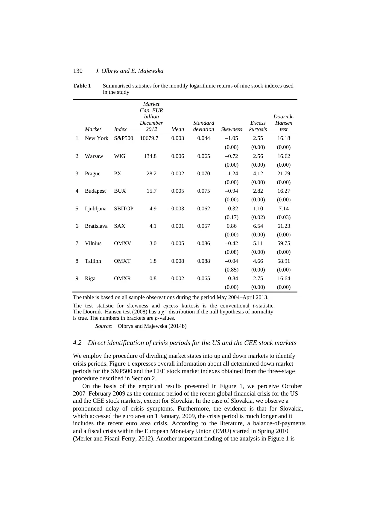
Table 1 reports summarised statistics for the monthly logarithmic returns for nine stock
indexes (in order of decreasing value of market capitalisation at the end of 2012), as well
as statistics testing for normality.
Several results in Table 1 are worth a comment. The measure for skewness shows that
the return series are skewed, except for the SBI TOP, OMXV and OMXT series.
The measure for excess kurtosis shows that all series are highly leptokurtic with respect
to the normal distribution. The Doornik-Hansen (Doornik and Hansen, 2008) test rejects
normality for each of the return series at the 5% level of significance.
hence δ ≥ 0 and ˆ ˆ ,VA Cρ ρ≤ i.e., during the periods of high volatility the unconditional
volatility-adjusted cross-correlation ˆVAρ will be smaller than the estimated conditional
cross-correlation ˆCρ between markets. The evaluation of contagion is carried out by
testing the hypotheses:
0
1
:
: ,
VA PC
VA PC
H
H
ρ ρ
ρ ρ
=
≠ (5)
where PCρ is the cross-correlation coefficient in the pre-crisis period, and the null
hypothesis states that there is no contagion. The Z-statistic, which is asymptotically a
standard normal random variable, tests the null of no contagion, i.e., the equality of the
crisis with pre-crisis cross-market correlation coefficients. The test is performed with the
Fisher (1921) z-transformation of sample correlation coefficients. If the absolute value of
the Z-statistic is greater than the critical value, the null hypothesis of identical correlation
coefficients can be rejected (Olbrys and Majewska, 2014c).
4 Data description and empirical results on the main indexes of the CEE
and US stock markets
In this study, we use our own database, not a commercial one. The raw data consists of
daily closing prices of the stock market indexes. We calculate daily, weekly and monthly
logarithmic returns of the major CEE stock market indexes (i.e., WIG, PX, BUX, SBI
TOP, SAX, OMXV, OMXT and OMXR) and the New York market index – S&P500.
There are 1969 daily, 469 weekly and 108 monthly observations for each series for the
period beginning May 2004 and ending April 2013 (9 years). To employ the procedure
described in Section 2, the data was extended to the period from September 2003 to
December 2013 (eight months back and forward).
We use weekly Wednesday-to-Wednesday logarithmic returns, which are thought to
iron out any possible impact of the day-of-the-week effects of daily data. As for daily
returns, one potentially serious problem, which may substantially disrupt various analyses
employing multivariate time series, is the non-synchronous trading effect II between
international stock markets (Olbrys and Majewska, 2014d). Therefore, in this research,
we employ a ‘common trading window’ procedure as a daily data-matching method. We
perform the robustness analysis with respect to various data frequencies, using daily,
weekly and monthly logarithmic returns of the stock market indexes. All analyses are
conducted using the open-source computer software Gretl 1.9.14 (Adkins, 2014).
4.1 Preliminary statistics
Table 1 reports summarised statistics for the monthly logarithmic returns for nine stock
indexes (in order of decreasing value of market capitalisation at the end of 2012), as well
as statistics testing for normality.
Several results in Table 1 are worth a comment. The measure for skewness shows that
the return series are skewed, except for the SBI TOP, OMXV and OMXT series.
The measure for excess kurtosis shows that all series are highly leptokurtic with respect
to the normal distribution. The Doornik-Hansen (Doornik and Hansen, 2008) test rejects
normality for each of the return series at the 5% level of significance.
Paraphrase This Document
Need a fresh take? Get an instant paraphrase of this document with our AI Paraphraser
130 J. Olbrys and E. Majewska
Table 1 Summarised statistics for the monthly logarithmic returns of nine stock indexes used
in the study
Market Index
Market
Cap. EUR
billion
December
2012 Mean
Standard
deviation Skewness
Excess
kurtosis
Doornik-
Hansen
test
1 New York S&P500 10679.7 0.003 0.044 –1.05 2.55 16.18
(0.00) (0.00) (0.00)
2 Warsaw WIG 134.8 0.006 0.065 –0.72 2.56 16.62
(0.00) (0.00) (0.00)
3 Prague PX 28.2 0.002 0.070 –1.24 4.12 21.79
(0.00) (0.00) (0.00)
4 Budapest BUX 15.7 0.005 0.075 –0.94 2.82 16.27
(0.00) (0.00) (0.00)
5 Ljubljana SBITOP 4.9 –0.003 0.062 –0.32 1.10 7.14
(0.17) (0.02) (0.03)
6 Bratislava SAX 4.1 0.001 0.057 0.86 6.54 61.23
(0.00) (0.00) (0.00)
7 Vilnius OMXV 3.0 0.005 0.086 –0.42 5.11 59.75
(0.08) (0.00) (0.00)
8 Tallinn OMXT 1.8 0.008 0.088 –0.04 4.66 58.91
(0.85) (0.00) (0.00)
9 Riga OMXR 0.8 0.002 0.065 –0.84 2.75 16.64
(0.00) (0.00) (0.00)
The table is based on all sample observations during the period May 2004–April 2013.
The test statistic for skewness and excess kurtosis is the conventional t-statistic.
The Doornik–Hansen test (2008) has a χ 2 distribution if the null hypothesis of normality
is true. The numbers in brackets are p-values.
Source: Olbrys and Majewska (2014b)
4.2 Direct identification of crisis periods for the US and the CEE stock markets
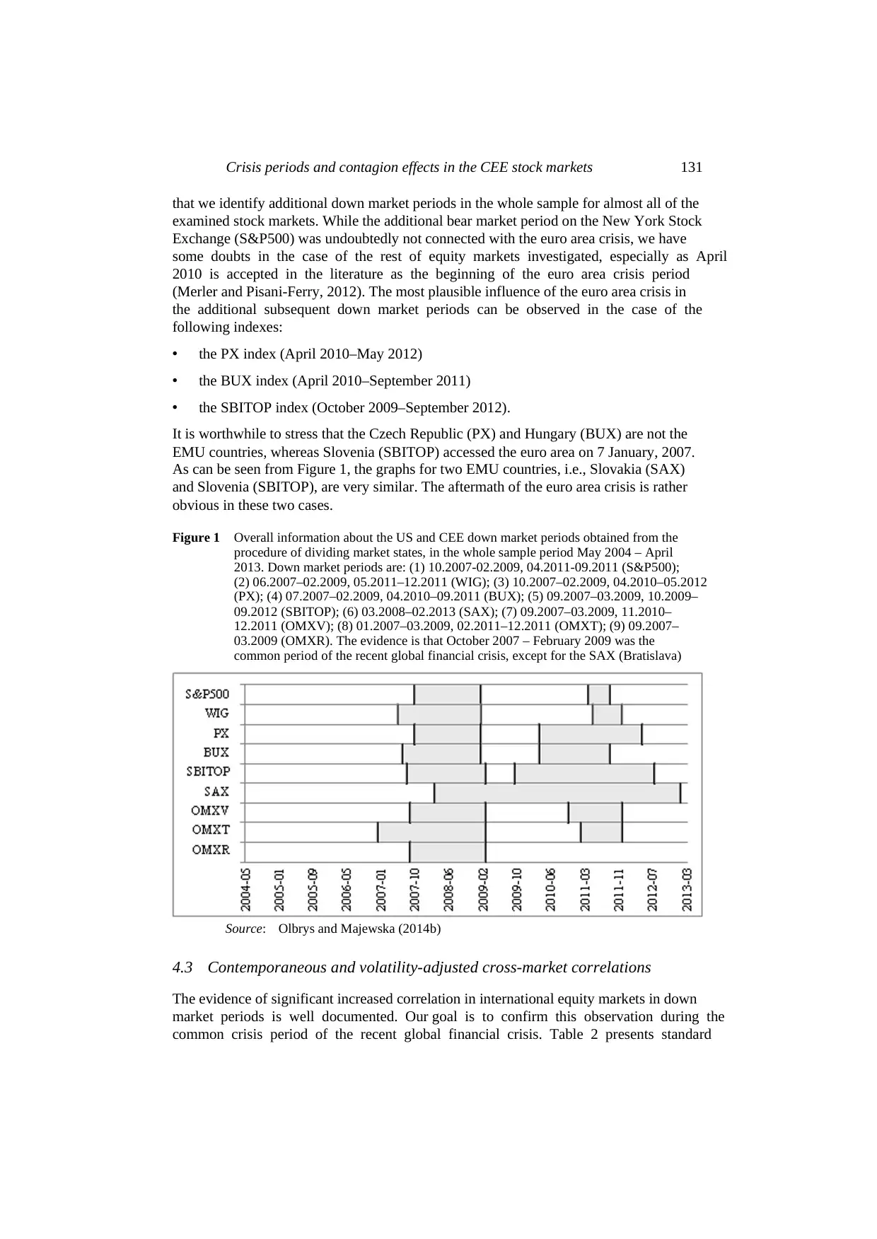
We employ the procedure of dividing market states into up and down markets to identify
crisis periods. Figure 1 expresses overall information about all determined down market
periods for the S&P500 and the CEE stock market indexes obtained from the three-stage
procedure described in Section 2.
On the basis of the empirical results presented in Figure 1, we perceive October
2007–February 2009 as the common period of the recent global financial crisis for the US
and the CEE stock markets, except for Slovakia. In the case of Slovakia, we observe a
pronounced delay of crisis symptoms. Furthermore, the evidence is that for Slovakia,
which accessed the euro area on 1 January, 2009, the crisis period is much longer and it
includes the recent euro area crisis. According to the literature, a balance-of-payments
and a fiscal crisis within the European Monetary Union (EMU) started in Spring 2010
(Merler and Pisani-Ferry, 2012). Another important finding of the analysis in Figure 1 is
Table 1 Summarised statistics for the monthly logarithmic returns of nine stock indexes used
in the study
Market Index
Market
Cap. EUR
billion
December
2012 Mean
Standard
deviation Skewness
Excess
kurtosis
Doornik-
Hansen
test
1 New York S&P500 10679.7 0.003 0.044 –1.05 2.55 16.18
(0.00) (0.00) (0.00)
2 Warsaw WIG 134.8 0.006 0.065 –0.72 2.56 16.62
(0.00) (0.00) (0.00)
3 Prague PX 28.2 0.002 0.070 –1.24 4.12 21.79
(0.00) (0.00) (0.00)
4 Budapest BUX 15.7 0.005 0.075 –0.94 2.82 16.27
(0.00) (0.00) (0.00)
5 Ljubljana SBITOP 4.9 –0.003 0.062 –0.32 1.10 7.14
(0.17) (0.02) (0.03)
6 Bratislava SAX 4.1 0.001 0.057 0.86 6.54 61.23
(0.00) (0.00) (0.00)
7 Vilnius OMXV 3.0 0.005 0.086 –0.42 5.11 59.75
(0.08) (0.00) (0.00)
8 Tallinn OMXT 1.8 0.008 0.088 –0.04 4.66 58.91
(0.85) (0.00) (0.00)
9 Riga OMXR 0.8 0.002 0.065 –0.84 2.75 16.64
(0.00) (0.00) (0.00)
The table is based on all sample observations during the period May 2004–April 2013.
The test statistic for skewness and excess kurtosis is the conventional t-statistic.
The Doornik–Hansen test (2008) has a χ 2 distribution if the null hypothesis of normality
is true. The numbers in brackets are p-values.
Source: Olbrys and Majewska (2014b)
4.2 Direct identification of crisis periods for the US and the CEE stock markets
We employ the procedure of dividing market states into up and down markets to identify
crisis periods. Figure 1 expresses overall information about all determined down market
periods for the S&P500 and the CEE stock market indexes obtained from the three-stage
procedure described in Section 2.
On the basis of the empirical results presented in Figure 1, we perceive October
2007–February 2009 as the common period of the recent global financial crisis for the US
and the CEE stock markets, except for Slovakia. In the case of Slovakia, we observe a
pronounced delay of crisis symptoms. Furthermore, the evidence is that for Slovakia,
which accessed the euro area on 1 January, 2009, the crisis period is much longer and it
includes the recent euro area crisis. According to the literature, a balance-of-payments
and a fiscal crisis within the European Monetary Union (EMU) started in Spring 2010
(Merler and Pisani-Ferry, 2012). Another important finding of the analysis in Figure 1 is
Crisis periods and contagion effects in the CEE stock markets 131
that we identify additional down market periods in the whole sample for almost all of the
examined stock markets. While the additional bear market period on the New York Stock
Exchange (S&P500) was undoubtedly not connected with the euro area crisis, we have
some doubts in the case of the rest of equity markets investigated, especially as April
2010 is accepted in the literature as the beginning of the euro area crisis period
(Merler and Pisani-Ferry, 2012). The most plausible influence of the euro area crisis in
the additional subsequent down market periods can be observed in the case of the
following indexes:
• the PX index (April 2010–May 2012)
• the BUX index (April 2010–September 2011)
• the SBITOP index (October 2009–September 2012).
It is worthwhile to stress that the Czech Republic (PX) and Hungary (BUX) are not the
EMU countries, whereas Slovenia (SBITOP) accessed the euro area on 7 January, 2007.
As can be seen from Figure 1, the graphs for two EMU countries, i.e., Slovakia (SAX)
and Slovenia (SBITOP), are very similar. The aftermath of the euro area crisis is rather
obvious in these two cases.
Figure 1 Overall information about the US and CEE down market periods obtained from the
procedure of dividing market states, in the whole sample period May 2004 – April
2013. Down market periods are: (1) 10.2007-02.2009, 04.2011-09.2011 (S&P500);
(2) 06.2007–02.2009, 05.2011–12.2011 (WIG); (3) 10.2007–02.2009, 04.2010–05.2012
(PX); (4) 07.2007–02.2009, 04.2010–09.2011 (BUX); (5) 09.2007–03.2009, 10.2009–
09.2012 (SBITOP); (6) 03.2008–02.2013 (SAX); (7) 09.2007–03.2009, 11.2010–
12.2011 (OMXV); (8) 01.2007–03.2009, 02.2011–12.2011 (OMXT); (9) 09.2007–
03.2009 (OMXR). The evidence is that October 2007 – February 2009 was the
common period of the recent global financial crisis, except for the SAX (Bratislava)
Source: Olbrys and Majewska (2014b)
4.3 Contemporaneous and volatility-adjusted cross-market correlations
The evidence of significant increased correlation in international equity markets in down
market periods is well documented. Our goal is to confirm this observation during the
common crisis period of the recent global financial crisis. Table 2 presents standard
⊘ This is a preview!⊘
Do you want full access?
Subscribe today to unlock all pages.
Trusted by 1+ million students worldwide
132 J. Olbrys and E. Majewska
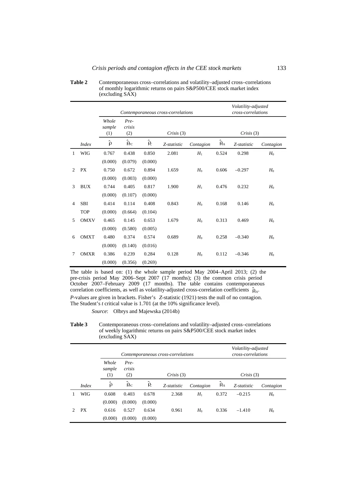
contemporaneous correlations and volatility-adjusted correlation coefficients, given by
equation (3), of monthly logarithmic returns on the pairs of indexes S&P500/CEE stock
market index (excluding SAX). For comparison, we calculate the dependencies both in
the whole sample (May 2004–April 2013) and in two subsamples of equal size:
• the pre-crisis period May 2006–September 2007 (17 months)
• the common crisis period October 2007–February 2009 (17 months).
We investigate the cross-market linkages after a shock to the US financial market.
Supporting values are equal to: 2
ˆCσ = 0.00362 (the variance in the high-volatility period
in the US stock market) and 2
ˆPCσ = 0.00053 (the variance in the low-volatility period in
the US stock market), while the relative increase in the variance of S&P500, given by
equation (4), is equal to δ = 5.8663. Our results confirm that during the period of high
volatility in the US stock market (the common crisis period October 2007–February
2009), the estimated conditional cross-correlations between the US and CEE markets
were greater than the corresponding unconditional volatility-adjusted correlations;
however, the p-values in brackets inform that contemporaneous correlations are not
statistically significant in some cases.
Several results in Table 2 are especially important. On the basis of the monthly
data, there is no reason to reject the null hypothesis of no contagion based on
volatility-adjusted cross-market correlations for each of the return series. The Student’s t
critical value is 1.701 (at the 10% level of significance). On the other hand, in the case
of contemporaneous cross-market correlations, the conclusions concerning contagion
are not such homogeneous. As we can observe, the Forbes-Rigobon correction for
heteroscedastic bias in index returns leads to a substantial reduction in differences among
cross-market correlation coefficients in the pre-crisis and crisis periods. Our results are
consistent with the literature and confirm that accommodating heteroscedasticity is valid
for detecting contagion across international stock markets (e.g., Forbes and Rigobon,
2002; Serwa and Bohl, 2005).
4.4 Robustness analysis of contagion tests
In this section, we present the robustness analysis of the empirical results concerning the
research hypothesis of no contagion effects among the US and the CEE equity markets
during the recent 2007–2009 global financial crisis. We perform contagion tests using
weekly and daily logarithmic returns and we compare the results obtained with those
presented in Table 2 for monthly returns.
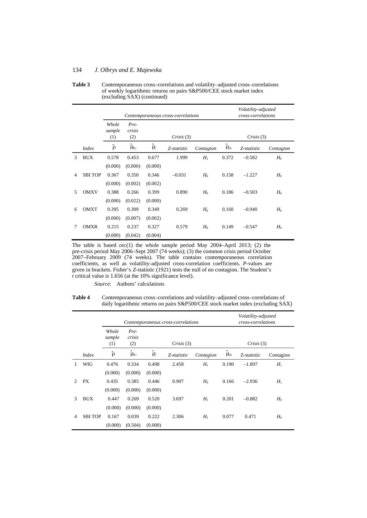
The empirical results reported in Tables 2–4 are not homogeneous, albeit only in a
few cases. On the one hand, the results of the testing of the null hypothesis of no
contagion effects based on both the monthly and the weekly data are qualitatively the
same (see Tables 2 and 3). On the other hand, when daily logarithmic returns are used
(Table 4), we observe that changes in the data frequency had some impact on the results
obtained. Unlike those shown in Tables 2–3, the results based on the Forbes-Rigobon
volatility-adjusted cross-market correlations allow to reject the null of no contagion for
daily logarithmic returns of the WIG (Warsaw) and PX (Prague) indexes. To sum up, the
results reveal that the contagion tests are rather less sensitive with respect to the choice of
data frequency.
contemporaneous correlations and volatility-adjusted correlation coefficients, given by
equation (3), of monthly logarithmic returns on the pairs of indexes S&P500/CEE stock
market index (excluding SAX). For comparison, we calculate the dependencies both in
the whole sample (May 2004–April 2013) and in two subsamples of equal size:
• the pre-crisis period May 2006–September 2007 (17 months)
• the common crisis period October 2007–February 2009 (17 months).
We investigate the cross-market linkages after a shock to the US financial market.
Supporting values are equal to: 2
ˆCσ = 0.00362 (the variance in the high-volatility period
in the US stock market) and 2
ˆPCσ = 0.00053 (the variance in the low-volatility period in
the US stock market), while the relative increase in the variance of S&P500, given by
equation (4), is equal to δ = 5.8663. Our results confirm that during the period of high
volatility in the US stock market (the common crisis period October 2007–February
2009), the estimated conditional cross-correlations between the US and CEE markets
were greater than the corresponding unconditional volatility-adjusted correlations;
however, the p-values in brackets inform that contemporaneous correlations are not
statistically significant in some cases.
Several results in Table 2 are especially important. On the basis of the monthly
data, there is no reason to reject the null hypothesis of no contagion based on
volatility-adjusted cross-market correlations for each of the return series. The Student’s t
critical value is 1.701 (at the 10% level of significance). On the other hand, in the case
of contemporaneous cross-market correlations, the conclusions concerning contagion
are not such homogeneous. As we can observe, the Forbes-Rigobon correction for
heteroscedastic bias in index returns leads to a substantial reduction in differences among
cross-market correlation coefficients in the pre-crisis and crisis periods. Our results are
consistent with the literature and confirm that accommodating heteroscedasticity is valid
for detecting contagion across international stock markets (e.g., Forbes and Rigobon,
2002; Serwa and Bohl, 2005).
4.4 Robustness analysis of contagion tests
In this section, we present the robustness analysis of the empirical results concerning the
research hypothesis of no contagion effects among the US and the CEE equity markets
during the recent 2007–2009 global financial crisis. We perform contagion tests using
weekly and daily logarithmic returns and we compare the results obtained with those
presented in Table 2 for monthly returns.
The empirical results reported in Tables 2–4 are not homogeneous, albeit only in a
few cases. On the one hand, the results of the testing of the null hypothesis of no
contagion effects based on both the monthly and the weekly data are qualitatively the
same (see Tables 2 and 3). On the other hand, when daily logarithmic returns are used
(Table 4), we observe that changes in the data frequency had some impact on the results
obtained. Unlike those shown in Tables 2–3, the results based on the Forbes-Rigobon
volatility-adjusted cross-market correlations allow to reject the null of no contagion for
daily logarithmic returns of the WIG (Warsaw) and PX (Prague) indexes. To sum up, the
results reveal that the contagion tests are rather less sensitive with respect to the choice of
data frequency.
Paraphrase This Document
Need a fresh take? Get an instant paraphrase of this document with our AI Paraphraser
Crisis periods and contagion effects in the CEE stock markets 133
Table 2 Contemporaneous cross–correlations and volatility–adjusted cross–correlations
of monthly logarithmic returns on pairs S&P500/CEE stock market index
(excluding SAX)
Index
Contemporaneous cross-correlations
Volatility-adjusted
cross-correlations
Whole
sample
(1)
Pre-
crisis
(2) Crisis (3) Crisis (3)
ˆρ ˆPCρ ˆCρ Z-statistic Contagion ˆVAρ Z-statistic Contagion
1 WIG 0.767 0.438 0.850 2.081 H1 0.524 0.298 H0
(0.000) (0.079) (0.000)
2 PX 0.750 0.672 0.894 1.659 H0 0.606 –0.297 H0
(0.000) (0.003) (0.000)
3 BUX 0.744 0.405 0.817 1.900 H1 0.476 0.232 H0
(0.000) (0.107) (0.000)
4 SBI 0.414 0.114 0.408 0.843 H0 0.168 0.146 H0
TOP (0.000) (0.664) (0.104)
5 OMXV 0.465 0.145 0.653 1.679 H0 0.313 0.469 H0
(0.000) (0.580) (0.005)
6 OMXT 0.480 0.374 0.574 0.689 H0 0.258 –0.340 H0
(0.000) (0.140) (0.016)
7 OMXR 0.386 0.239 0.284 0.128 H0 0.112 –0.346 H0
(0.000) (0.356) (0.269)
The table is based on: (1) the whole sample period May 2004–April 2013; (2) the
pre-crisis period May 2006–Sept 2007 (17 months); (3) the common crisis period
October 2007–February 2009 (17 months). The table contains contemporaneous
correlation coefficients, as well as volatility-adjusted cross-correlation coefficients ˆ .VAρ
P-values are given in brackets. Fisher’s Z-statistic (1921) tests the null of no contagion.
The Student’s t critical value is 1.701 (at the 10% significance level).
Source: Olbrys and Majewska (2014b)
Table 3 Contemporaneous cross–correlations and volatility–adjusted cross–correlations
of weekly logarithmic returns on pairs S&P500/CEE stock market index
(excluding SAX)
Index
Contemporaneous cross-correlations
Volatility-adjusted
cross-correlations
Whole
sample
(1)
Pre-
crisis
(2) Crisis (3) Crisis (3)
ˆρ ˆPCρ ˆCρ Z-statistic Contagion ˆVAρ Z-statistic Contagion
1 WIG 0.608 0.403 0.678 2.368 H1 0.372 –0.215 H0
(0.000) (0.000) (0.000)
2 PX 0.616 0.527 0.634 0.961 H0 0.336 –1.410 H0
(0.000) (0.000) (0.000)
134 J. Olbrys and E. Majewska
Table 3 Contemporaneous cross–correlations and volatility–adjusted cross–correlations
of weekly logarithmic returns on pairs S&P500/CEE stock market index
(excluding SAX) (continued)
Index
Contemporaneous cross-correlations
Volatility-adjusted
cross-correlations
Whole
sample
(1)
Pre-
crisis
(2) Crisis (3) Crisis (3)
ˆρ ˆPCρ ˆCρ Z-statistic Contagion ˆVAρ Z-statistic Contagion
3 BUX 0.578 0.453 0.677 1.999 H1 0.372 –0.582 H0
(0.000) (0.000) (0.000)
4 SBI TOP 0.367 0.350 0.346 –0.031 H0 0.158 –1.227 H0
(0.000) (0.002) (0.002)
5 OMXV 0.388 0.266 0.399 0.890 H0 0.186 –0.503 H0
(0.000) (0.022) (0.000)
6 OMXT 0.395 0.309 0.349 0.269 H0 0.160 –0.940 H0
(0.000) (0.007) (0.002)
7 OMXR 0.215 0.237 0.327 0.579 H0 0.149 –0.547 H0
(0.000) (0.042) (0.004)
The table is based on:(1) the whole sample period May 2004–April 2013; (2) the
pre-crisis period May 2006–Sept 2007 (74 weeks); (3) the common crisis period October
2007–February 2009 (74 weeks). The table contains contemporaneous correlation
coefficients, as well as volatility-adjusted cross-correlation coefficients. P-values are
given in brackets. Fisher’s Z-statistic (1921) tests the null of no contagion. The Student’s
t critical value is 1.656 (at the 10% significance level).
Source: Authors’ calculations
Table 4 Contemporaneous cross–correlations and volatility–adjusted cross–correlations of
daily logarithmic returns on pairs S&P500/CEE stock market index (excluding SAX)
Contemporaneous cross-correlations
Volatility-adjusted
cross-correlations
Whole
sample
(1)
Pre-
crisis
(2) Crisis (3) Crisis (3)
Index ˆρ ˆPCρ ˆCρ Z-statistic Contagion ˆVAρ Z-statistic Contagion
1 WIG 0.476 0.334 0.498 2.458 H1 0.190 –1.897 H1
(0.000) (0.000) (0.000)
2 PX 0.435 0.385 0.446 0.907 H0 0.166 –2.936 H1
(0.000) (0.000) (0.000)
3 BUX 0.447 0.269 0.520 3.697 H1 0.201 –0.882 H0
(0.000) (0.000) (0.000)
4 SBI TOP 0.167 0.039 0.222 2.306 H1 0.077 0.471 H0
(0.000) (0.504) (0.000)
⊘ This is a preview!⊘
Do you want full access?
Subscribe today to unlock all pages.
Trusted by 1+ million students worldwide
1 out of 15
Your All-in-One AI-Powered Toolkit for Academic Success.
+13062052269
info@desklib.com
Available 24*7 on WhatsApp / Email
![[object Object]](/_next/static/media/star-bottom.7253800d.svg)
Unlock your academic potential
Copyright © 2020–2026 A2Z Services. All Rights Reserved. Developed and managed by ZUCOL.