Comprehensive Statistical Analysis of Financial Earnings and Data

This report presents a comprehensive analysis of financial statistics, focusing on earnings comparisons between men and women in both public and private sectors. The report utilizes t-tests to determine the significance of earnings differences, time charts to visualize annual income trends, and calculations for annual earning growth rates. Furthermore, it includes the estimation of median hourly earnings and quartiles using the ogive method, as well as the calculation of mean and standard deviation. The analysis extends to comparing earnings between Manchester and London, and designing bar and pie charts to support the data. The report delves into statistical methods such as t-tests, ogive method, mean, and standard deviation to provide a detailed understanding of financial data. The analysis includes interpretation of the results and the implications of various findings.

Statistics Financial

Table of Contents
INTRODUCTION...........................................................................................................................3
MAIN BODY...................................................................................................................................3
TASK 1............................................................................................................................................3
A) Comparison of the earnings of women and men in public sector...........................................3
B) Comparison of the earnings of women and men in private sector..........................................4
C) Presentation of earnings of different sector by Time chart method........................................5
D) Determination of annual earning growth rate.........................................................................6
TASK 2............................................................................................................................................7
A) ................................................................................................................................................7
1) Estimation of median hourly earning and quartiles by ogive method.....................................7
2) Calculation for mean and standard deviation..........................................................................9
B) Comparison of the earnings..................................................................................................10
TASK 3 .........................................................................................................................................11
Section A....................................................................................................................................11
Section B....................................................................................................................................11
TASK 4..........................................................................................................................................12
4.1...............................................................................................................................................12
1. Bar chart.................................................................................................................................12
2. Pie chart.................................................................................................................................15
....................................................................................................................................................17
4.2 Relationship between the number of bedrooms and the house price of bedrooms in all of
the three streets..........................................................................................................................18
CONCLUSION..............................................................................................................................24
REFERENCES..............................................................................................................................25

INTRODUCTION
The term financial statistics is related with all the numerical figures, data and values
which helps in summarizing relevant as well as appropriate information. Data as gathered with
the help of different statistical means is required to be evaluated with the help of the best tools
and methods for deriving proper interpretation from it. The present report is related with the use
of different statistical tools for assessing results out of it. This report will help in assessing
earnings of both the men and women of public & private sector with the help of hypothesis
made. Also, various charts and graphs will be presented for supporting such table made.
Furthermore, analysis of hourly pay rate in different region of UK will be provided. Also,
explanation related to economic order quantity along with requisite calculations made. At last the
report will also shed light on designing of both the bar and pie chart for supporting data of
different streets.
MAIN BODY
TASK 1
A) Comparison of the earnings of women and men in public sector
Null hypothesis H0 : There is no significance difference in the earning of both women and men
who work in public sector.
Alternative Hypothesis H1 : There is significance difference in the earnings of both women and
men who work in public sector.
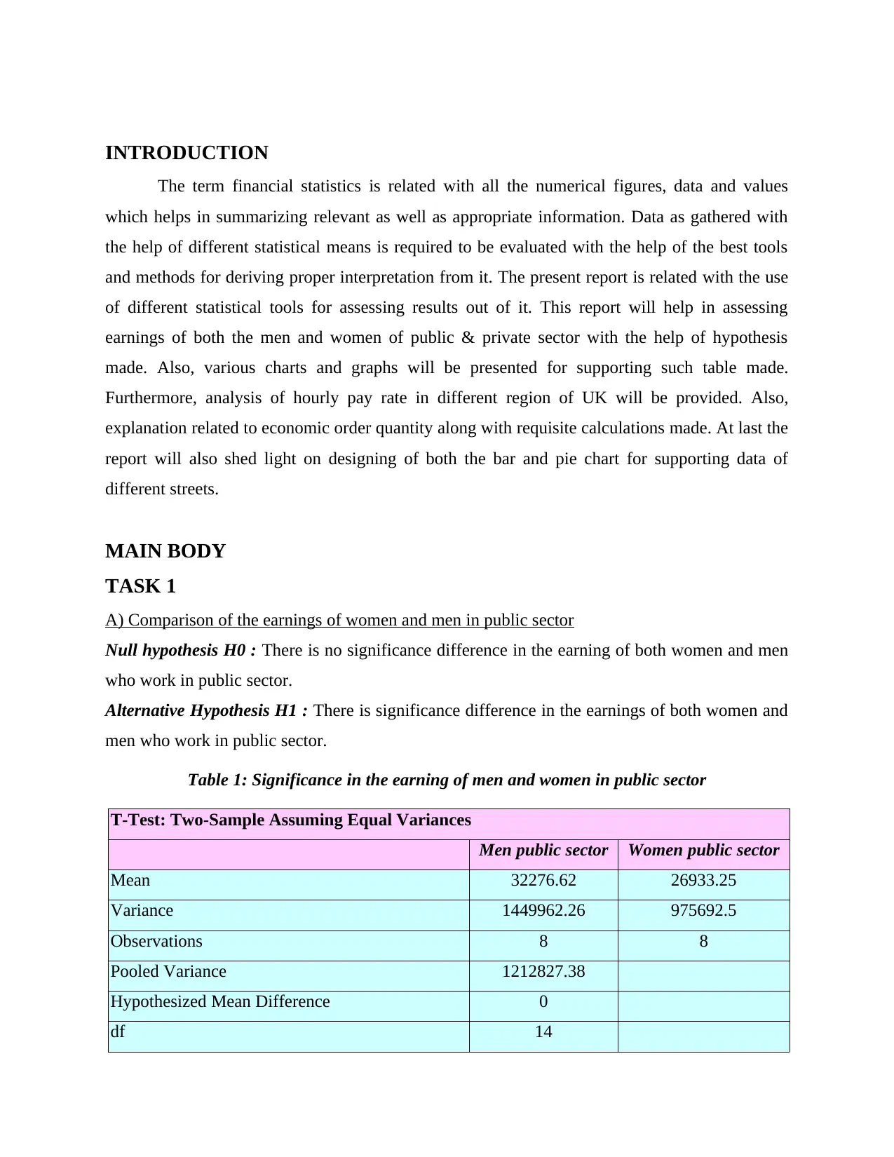
Table 1: Significance in the earning of men and women in public sector
T-Test: Two-Sample Assuming Equal Variances
Men public sector Women public sector
Mean 32276.62 26933.25
Variance 1449962.26 975692.5
Observations 8 8
Pooled Variance 1212827.38
Hypothesized Mean Difference 0
df 14

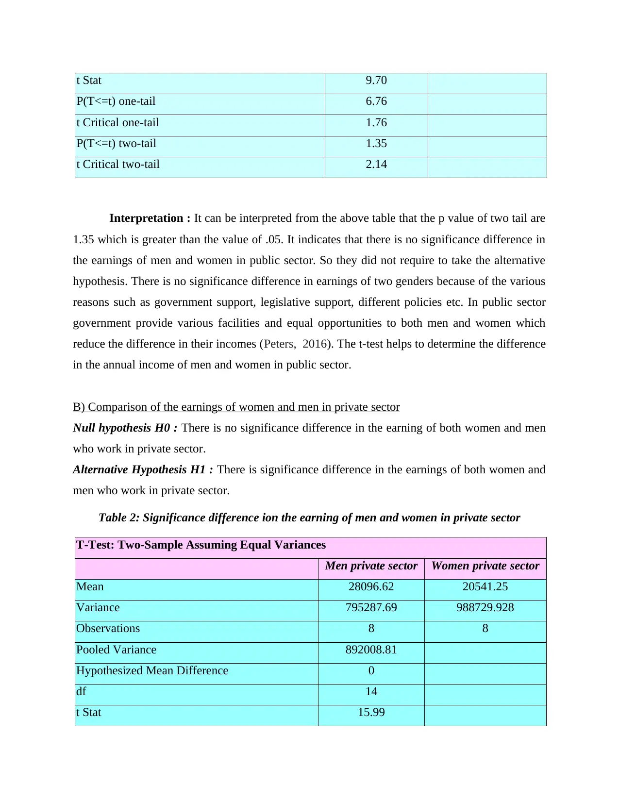
t Stat 9.70
P(T<=t) one-tail 6.76
t Critical one-tail 1.76
P(T<=t) two-tail 1.35
t Critical two-tail 2.14
Interpretation : It can be interpreted from the above table that the p value of two tail are
1.35 which is greater than the value of .05. It indicates that there is no significance difference in
the earnings of men and women in public sector. So they did not require to take the alternative
hypothesis. There is no significance difference in earnings of two genders because of the various
reasons such as government support, legislative support, different policies etc. In public sector
government provide various facilities and equal opportunities to both men and women which
reduce the difference in their incomes (Peters, 2016). The t-test helps to determine the difference
in the annual income of men and women in public sector.
B) Comparison of the earnings of women and men in private sector
Null hypothesis H0 : There is no significance difference in the earning of both women and men
who work in private sector.
Alternative Hypothesis H1 : There is significance difference in the earnings of both women and
men who work in private sector.
Table 2: Significance difference ion the earning of men and women in private sector
T-Test: Two-Sample Assuming Equal Variances
Men private sector Women private sector
Mean 28096.62 20541.25
Variance 795287.69 988729.928
Observations 8 8
Pooled Variance 892008.81
Hypothesized Mean Difference 0
df 14
t Stat 15.99

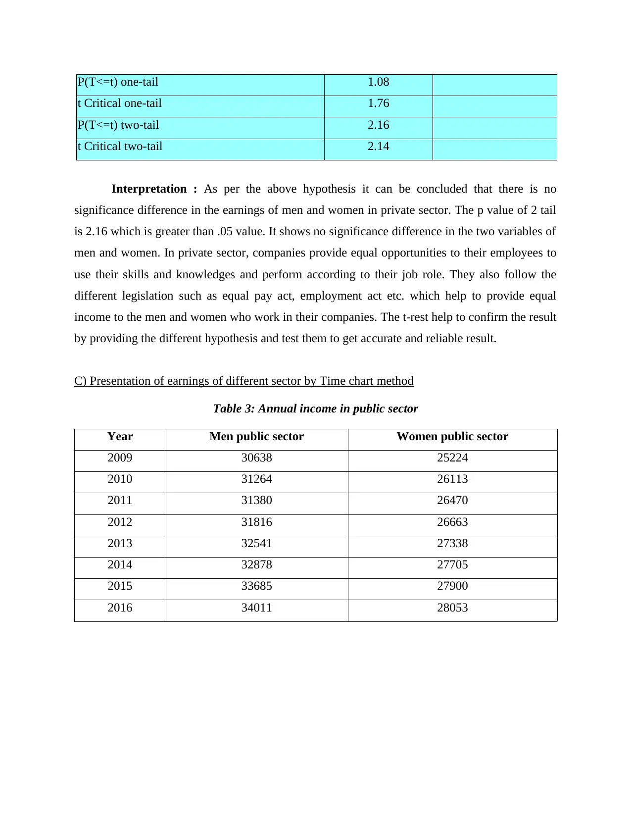
P(T<=t) one-tail 1.08
t Critical one-tail 1.76
P(T<=t) two-tail 2.16
t Critical two-tail 2.14
Interpretation : As per the above hypothesis it can be concluded that there is no
significance difference in the earnings of men and women in private sector. The p value of 2 tail
is 2.16 which is greater than .05 value. It shows no significance difference in the two variables of
men and women. In private sector, companies provide equal opportunities to their employees to
use their skills and knowledges and perform according to their job role. They also follow the
different legislation such as equal pay act, employment act etc. which help to provide equal
income to the men and women who work in their companies. The t-rest help to confirm the result
by providing the different hypothesis and test them to get accurate and reliable result.
C) Presentation of earnings of different sector by Time chart method
Table 3: Annual income in public sector
Year Men public sector Women public sector
2009 30638 25224
2010 31264 26113
2011 31380 26470
2012 31816 26663
2013 32541 27338
2014 32878 27705
2015 33685 27900
2016 34011 28053

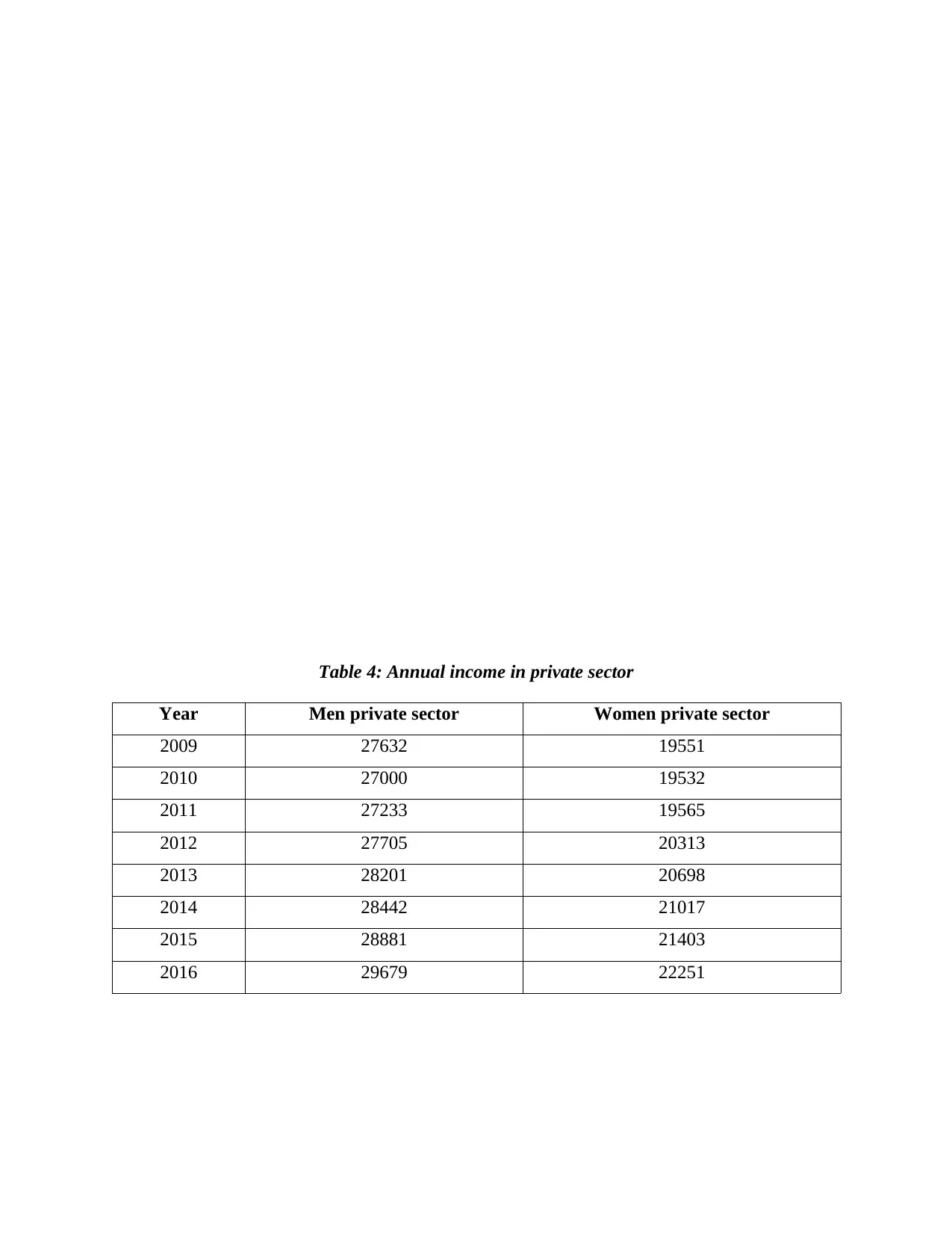
Table 4: Annual income in private sector
Year Men private sector Women private sector
2009 27632 19551
2010 27000 19532
2011 27233 19565
2012 27705 20313
2013 28201 20698
2014 28442 21017
2015 28881 21403
2016 29679 22251

1
2
3
4
5
6
7
8
0
20000
40000
Men and women in private sector
Men private sector Women private sector
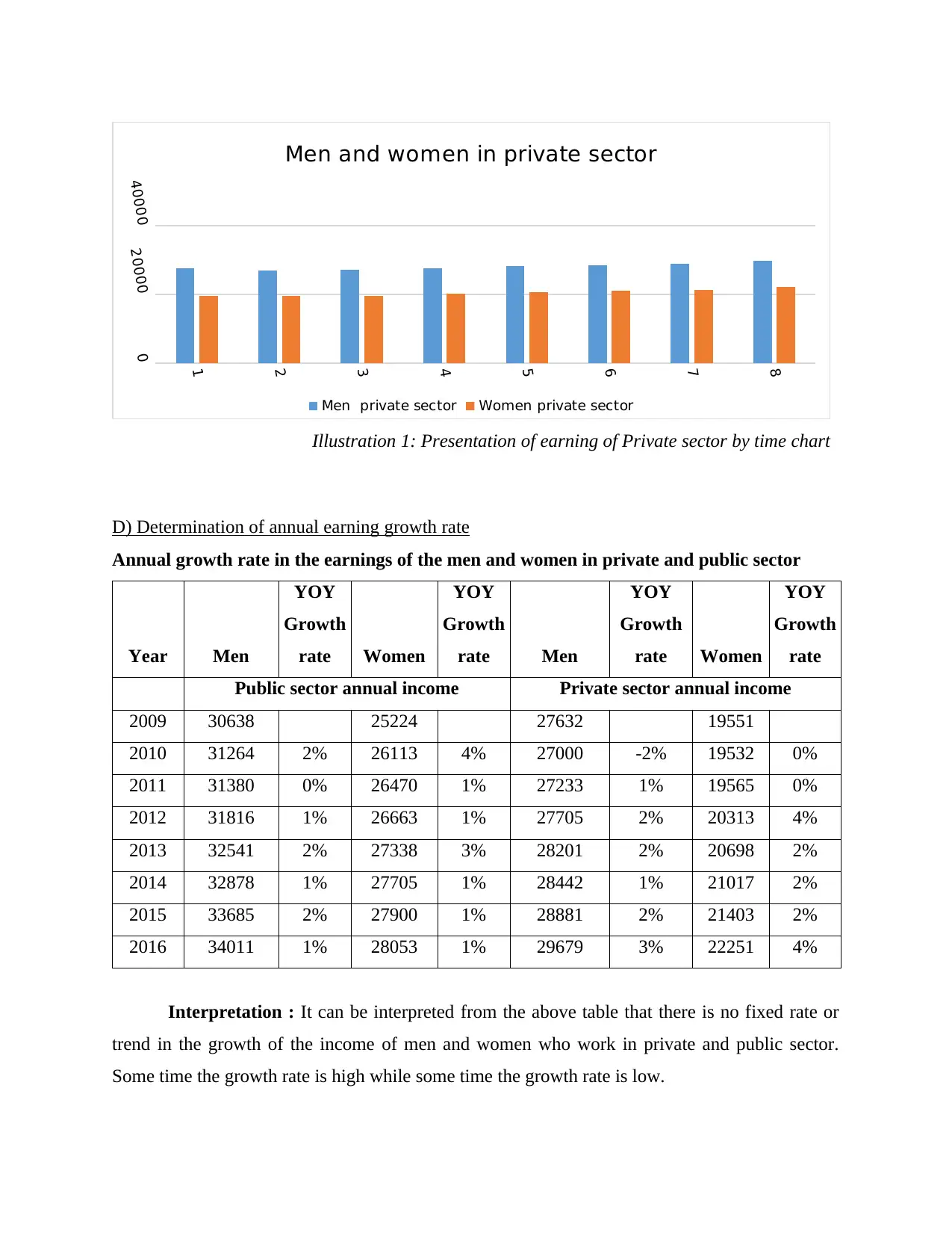
Illustration 1: Presentation of earning of Private sector by time chart
D) Determination of annual earning growth rate
Annual growth rate in the earnings of the men and women in private and public sector
Year Men
YOY
Growth
rate Women
YOY
Growth
rate Men
YOY
Growth
rate Women
YOY
Growth
rate
Public sector annual income Private sector annual income
2009 30638 25224 27632 19551
2010 31264 2% 26113 4% 27000 -2% 19532 0%
2011 31380 0% 26470 1% 27233 1% 19565 0%
2012 31816 1% 26663 1% 27705 2% 20313 4%
2013 32541 2% 27338 3% 28201 2% 20698 2%
2014 32878 1% 27705 1% 28442 1% 21017 2%
2015 33685 2% 27900 1% 28881 2% 21403 2%
2016 34011 1% 28053 1% 29679 3% 22251 4%
Interpretation : It can be interpreted from the above table that there is no fixed rate or
trend in the growth of the income of men and women who work in private and public sector.
Some time the growth rate is high while some time the growth rate is low.

TASK 2
A)
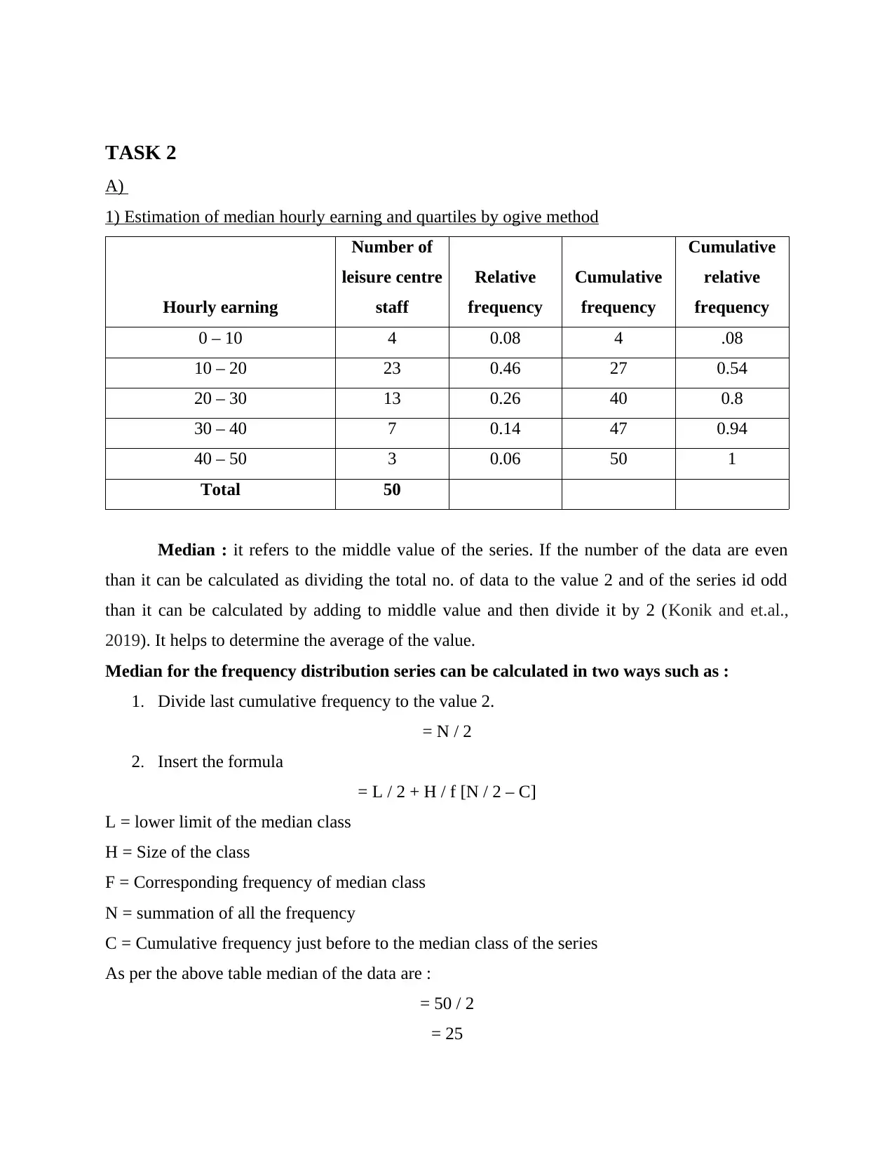
1) Estimation of median hourly earning and quartiles by ogive method
Hourly earning
Number of
leisure centre
staff
Relative
frequency
Cumulative
frequency
Cumulative
relative
frequency
0 – 10 4 0.08 4 .08
10 – 20 23 0.46 27 0.54
20 – 30 13 0.26 40 0.8
30 – 40 7 0.14 47 0.94
40 – 50 3 0.06 50 1
Total 50
Median : it refers to the middle value of the series. If the number of the data are even
than it can be calculated as dividing the total no. of data to the value 2 and of the series id odd
than it can be calculated by adding to middle value and then divide it by 2 (Konik and et.al.,
2019). It helps to determine the average of the value.
Median for the frequency distribution series can be calculated in two ways such as :
1. Divide last cumulative frequency to the value 2.
= N / 2
2. Insert the formula
= L / 2 + H / f [N / 2 – C]
L = lower limit of the median class
H = Size of the class
F = Corresponding frequency of median class
N = summation of all the frequency
C = Cumulative frequency just before to the median class of the series
As per the above table median of the data are :
= 50 / 2
= 25

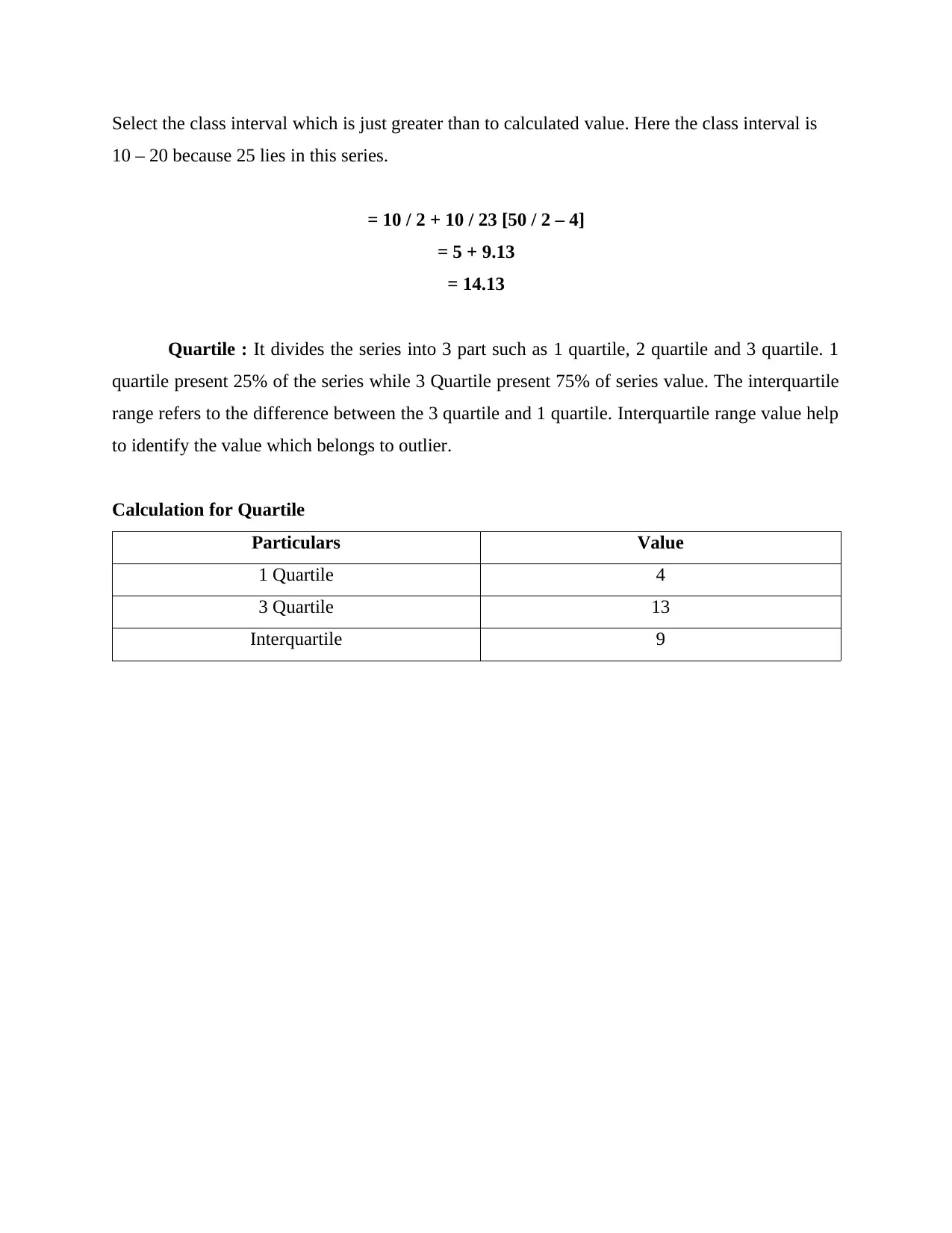
Select the class interval which is just greater than to calculated value. Here the class interval is
10 – 20 because 25 lies in this series.
= 10 / 2 + 10 / 23 [50 / 2 – 4]
= 5 + 9.13
= 14.13
Quartile : It divides the series into 3 part such as 1 quartile, 2 quartile and 3 quartile. 1
quartile present 25% of the series while 3 Quartile present 75% of series value. The interquartile
range refers to the difference between the 3 quartile and 1 quartile. Interquartile range value help
to identify the value which belongs to outlier.
Calculation for Quartile
Particulars Value
1 Quartile 4
3 Quartile 13
Interquartile 9

0 – 10 10 – 20 20 – 30 30 – 40 40 – 50
0
0.2
0.4
0.6
0.8
1
1.2
0.08
0.46
0.26
0.14
0.060.08
0.54
0.8
0.94 1
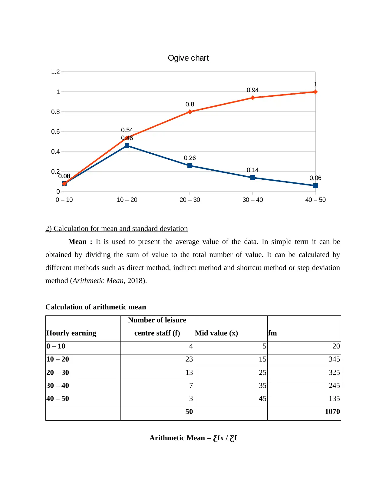
Ogive chart
2) Calculation for mean and standard deviation
Mean : It is used to present the average value of the data. In simple term it can be
obtained by dividing the sum of value to the total number of value. It can be calculated by
different methods such as direct method, indirect method and shortcut method or step deviation
method (Arithmetic Mean, 2018).
Calculation of arithmetic mean
Hourly earning
Number of leisure
centre staff (f) Mid value (x) fm
0 – 10 4 5 20
10 – 20 23 15 345
20 – 30 13 25 325
30 – 40 7 35 245
40 – 50 3 45 135
50 1070
Arithmetic Mean = Ƹfx / Ƹf

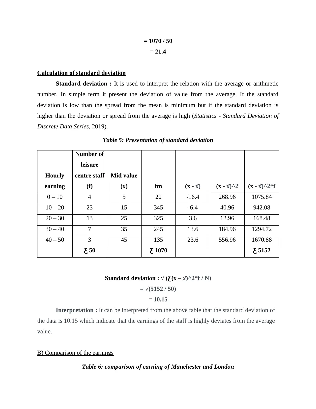
= 1070 / 50
= 21.4
Calculation of standard deviation
Standard deviation : It is used to interpret the relation with the average or arithmetic
number. In simple term it present the deviation of value from the average. If the standard
deviation is low than the spread from the mean is minimum but if the standard deviation is
higher than the deviation or spread from the average is high (Statistics - Standard Deviation of
Discrete Data Series, 2019).
Table 5: Presentation of standard deviation
Hourly
earning
Number of
leisure
centre staff
(f)
Mid value
(x) fm (x - x̄) (x - x̄)^2 (x - x̄)^2*f
0 – 10 4 5 20 -16.4 268.96 1075.84
10 – 20 23 15 345 -6.4 40.96 942.08
20 – 30 13 25 325 3.6 12.96 168.48
30 – 40 7 35 245 13.6 184.96 1294.72
40 – 50 3 45 135 23.6 556.96 1670.88
Ƹ 50 Ƹ 1070 Ƹ 5152
Standard deviation : √ (Ƹ(x – x̄)^2*f / N)
= √(5152 / 50)
= 10.15
Interpretation : It can be interpreted from the above table that the standard deviation of
the data is 10.15 which indicate that the earnings of the staff is highly deviates from the average
value.
B) Comparison of the earnings
Table 6: comparison of earning of Manchester and London

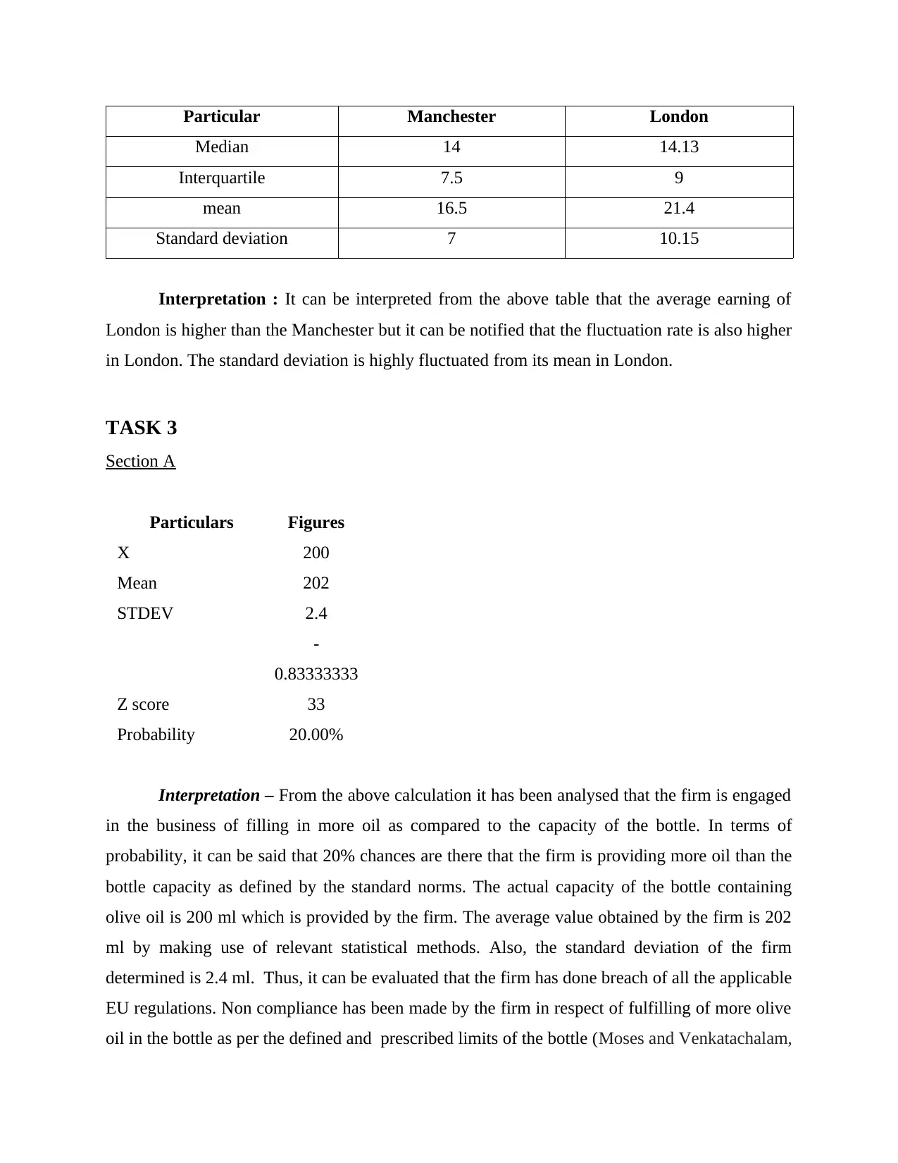
Particular Manchester London
Median 14 14.13
Interquartile 7.5 9
mean 16.5 21.4
Standard deviation 7 10.15
Interpretation : It can be interpreted from the above table that the average earning of
London is higher than the Manchester but it can be notified that the fluctuation rate is also higher
in London. The standard deviation is highly fluctuated from its mean in London.
TASK 3
Section A
Particulars Figures
X 200
Mean 202
STDEV 2.4
Z score
-
0.83333333
33
Probability 20.00%
Interpretation – From the above calculation it has been analysed that the firm is engaged
in the business of filling in more oil as compared to the capacity of the bottle. In terms of
probability, it can be said that 20% chances are there that the firm is providing more oil than the
bottle capacity as defined by the standard norms. The actual capacity of the bottle containing
olive oil is 200 ml which is provided by the firm. The average value obtained by the firm is 202
ml by making use of relevant statistical methods. Also, the standard deviation of the firm
determined is 2.4 ml. Thus, it can be evaluated that the firm has done breach of all the applicable
EU regulations. Non compliance has been made by the firm in respect of fulfilling of more olive
oil in the bottle as per the defined and prescribed limits of the bottle (Moses and Venkatachalam,