BUS105 Computing Assignment: Financial Data Analysis and Report

This computing assignment for BUS105 analyzes financial data using various statistical methods. It begins with a data scatter plot exploring the relationship between income and annual contribution, determining the annual contribution for a specific income level and calculating z-scores. The assignment then delves into pivot tables to assess the relationship between investment risk (high vs. low) and loss/profit, calculating proportions and p-values to test hypotheses. Further analysis involves box and whisker plots to compare returns for risky and safe investments, followed by the calculation of confidence intervals. Finally, the assignment explores mean and standard deviation computations in finance, demonstrating their application in portfolio theory to determine the risk-return profile of different securities and make investment choices based on the coefficient of variation. The assignment uses Excel functions and provides a practical example of calculating mean and standard deviation from historical data.

Computing Assignment
Bus105
Student id
[Pick the date]

Section 1
Data
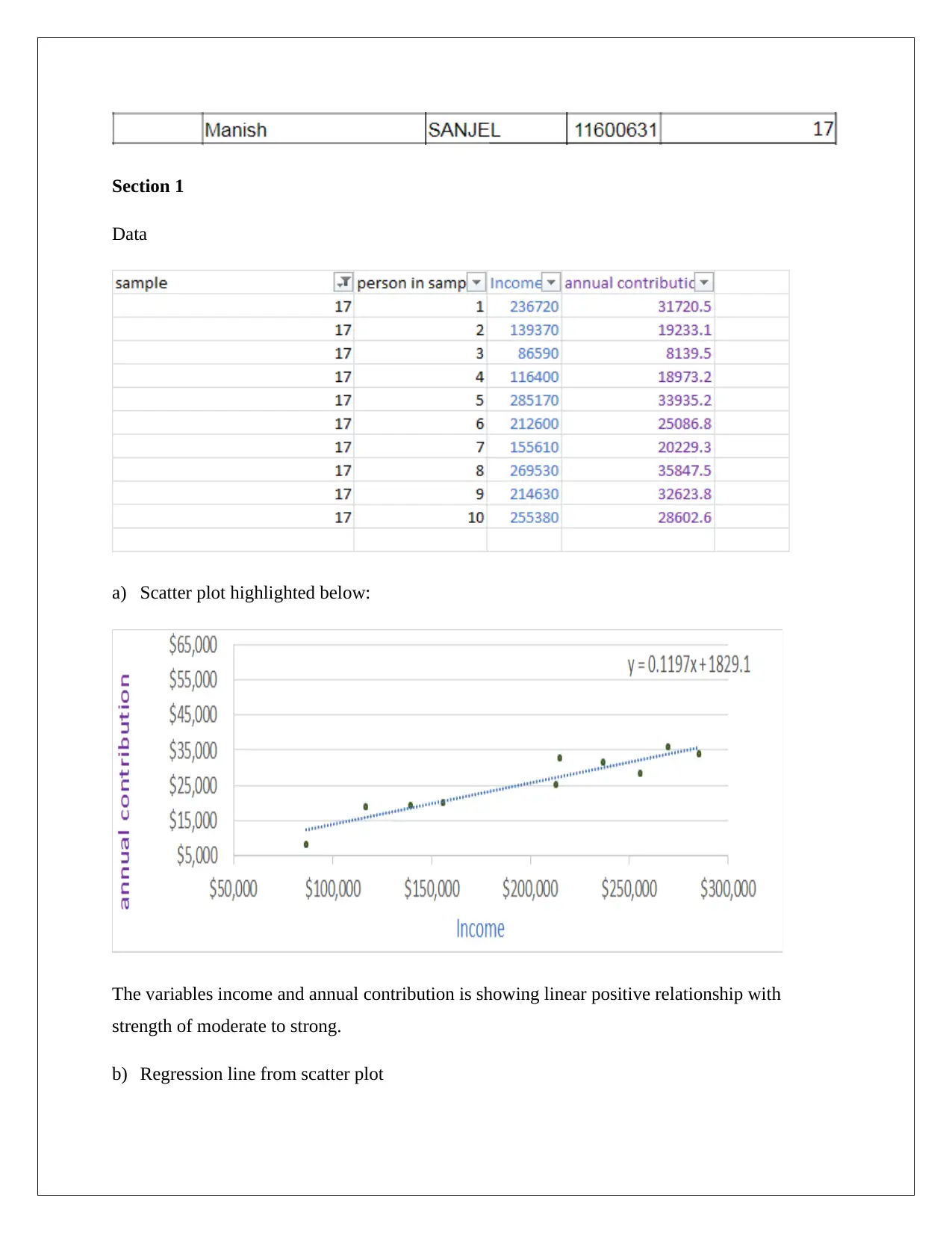
a) Scatter plot highlighted below:
The variables income and annual contribution is showing linear positive relationship with
strength of moderate to strong.
b) Regression line from scatter plot

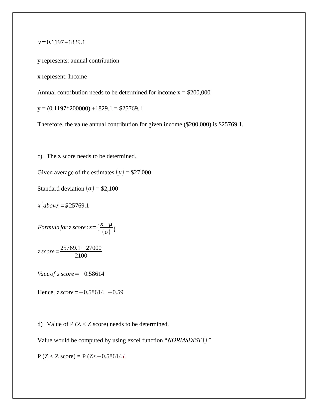
y=0.1197+1829.1
y represents: annual contribution
x represent: Income
Annual contribution needs to be determined for income x = $200,000
y = (0.1197*200000) +1829.1 = $25769.1
Therefore, the value annual contribution for given income ($200,000) is $25769.1.
c) The z score needs to be determined.
Given average of the estimates (μ) = $27,000
Standard deviation (σ ) = $2,100
x ( above ) =$ 25769.1
Formula for z score : z={ x−μ
(σ) }
z score=25769.1−27000
2100
Vaue of z score=−0.58614
Hence, z score=−0.58614 −0.59
d) Value of P (Z < Z score) needs to be determined.
Value would be computed by using excel function “NORMSDIST () ”
P (Z < Z score) = P (Z<−0.58614 ¿

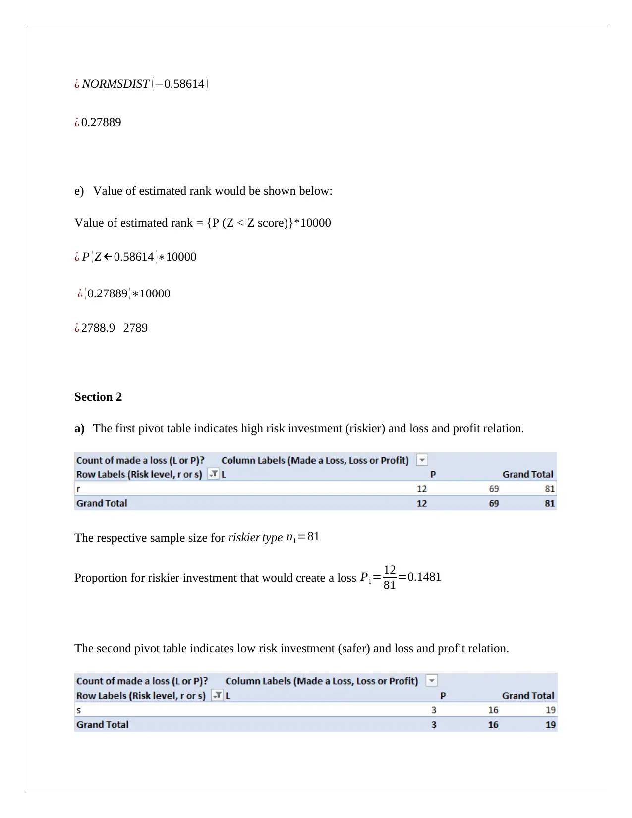
¿ NORMSDIST ( −0.58614 )
¿ 0.27889
e) Value of estimated rank would be shown below:
Value of estimated rank = {P (Z < Z score)}*10000
¿ P ( Z ←0.58614 )∗10000
¿ ( 0.27889 ) ∗10000
¿ 2788.9 2789
Section 2
a) The first pivot table indicates high risk investment (riskier) and loss and profit relation.
The respective sample size for riskier type n1=81
Proportion for riskier investment that would create a loss P1= 12
81 =0.1481
The second pivot table indicates low risk investment (safer) and loss and profit relation.

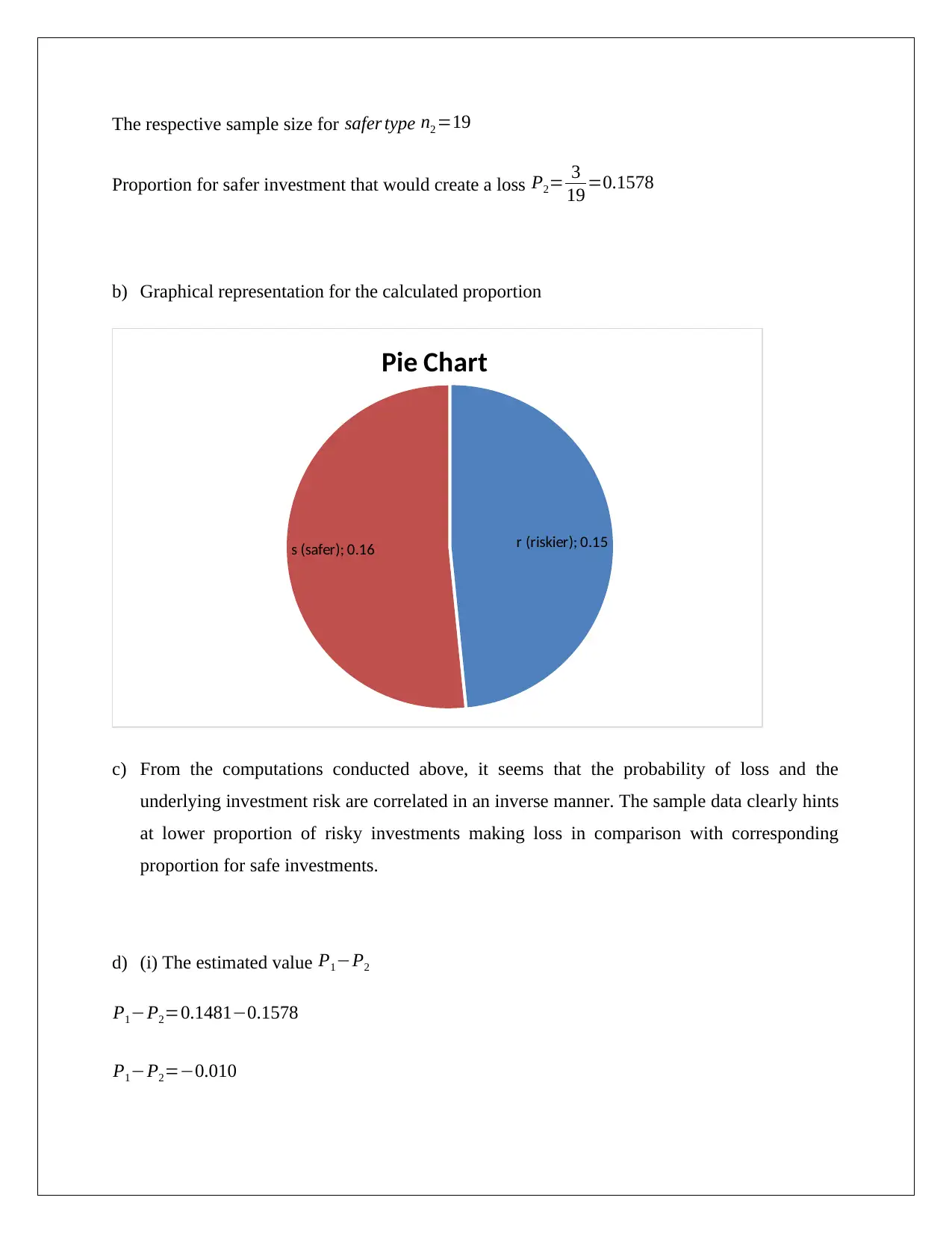
The respective sample size for safer type n2 =19
Proportion for safer investment that would create a loss P2= 3
19 =0.1578
b) Graphical representation for the calculated proportion
r (riskier); 0.15
s (safer); 0.16
Pie Chart
c) From the computations conducted above, it seems that the probability of loss and the
underlying investment risk are correlated in an inverse manner. The sample data clearly hints
at lower proportion of risky investments making loss in comparison with corresponding
proportion for safe investments.
d) (i) The estimated value P1−P2
P1−P2=0.1481−0.1578
P1−P2=−0.010

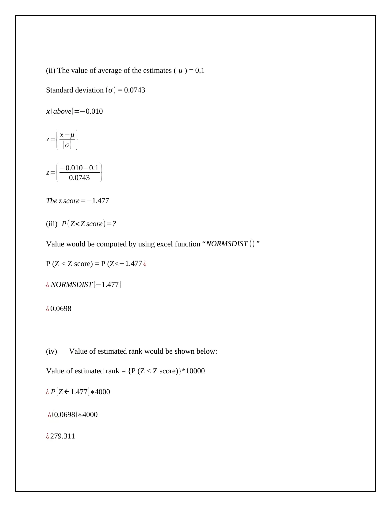
(ii) The value of average of the estimates ( μ ) = 0.1
Standard deviation (σ ) = 0.0743
x ( above ) =−0.010
z= { x −μ
( σ ) }
z= { −0.010−0.1
0.0743 }
The z score=−1.477
(iii) P( Z<Z score)=?
Value would be computed by using excel function “NORMSDIST () ”
P (Z < Z score) = P (Z< −1.477 ¿
¿ NORMSDIST (−1.477 )
¿ 0.0698
(iv) Value of estimated rank would be shown below:
Value of estimated rank = {P (Z < Z score)}*10000
¿ P ( Z ←1.477 )∗4000
¿ ( 0.0698 )∗4000
¿ 279.311

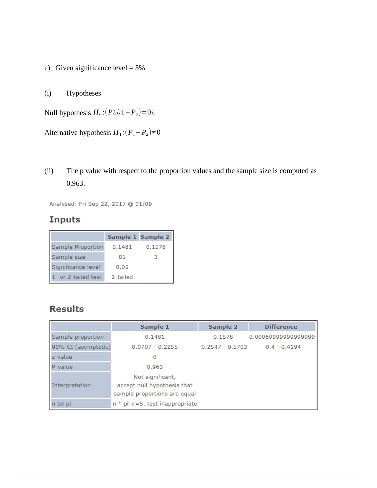
e) Given significance level = 5%
(i) Hypotheses
Null hypothesis H0 :(P¿¿ 1−P2)=0¿
Alternative hypothesis H1 :(P1−P2 )≠ 0
(ii) The p value with respect to the proportion values and the sample size is computed as
0.963.

(iii) It is apparent from the above output than p value is 0.963 which is higher than level of
significance and hence, insufficient statistical evidence is present to reject null
hypothesis.
(iv) Hence, it may be concluded that no relationship is observed between the investment
making loss and their underlying risk.
Section 3
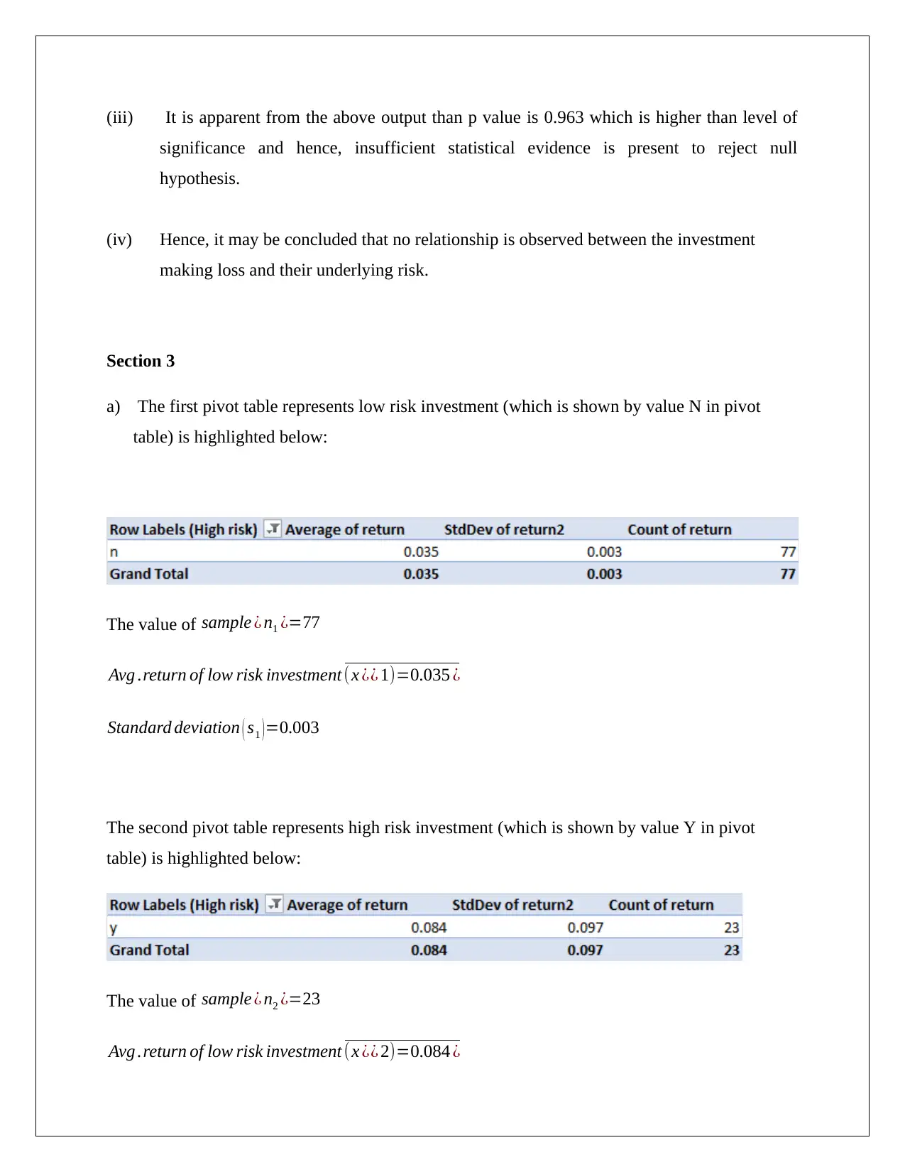
a) The first pivot table represents low risk investment (which is shown by value N in pivot
table) is highlighted below:
The value of sample ¿ n1 ¿=77
Avg .return of low risk investment (x ¿¿ 1)=0.035 ¿
Standard deviation ( s1 ) =0.003
The second pivot table represents high risk investment (which is shown by value Y in pivot
table) is highlighted below:
The value of sample ¿ n2 ¿=23
Avg .return of low risk investment (x ¿¿ 2)=0.084 ¿

Standard deviation(s2 )=0.097
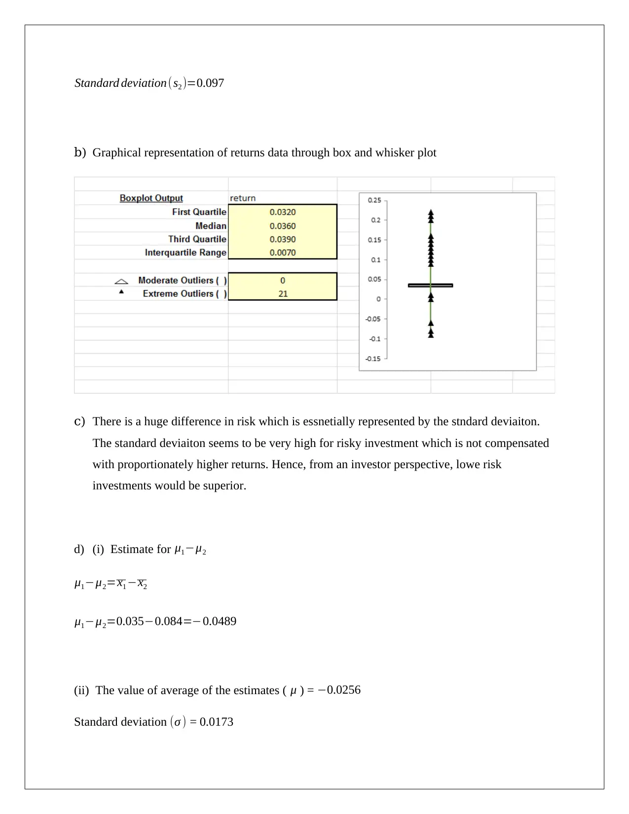
b) Graphical representation of returns data through box and whisker plot
c) There is a huge difference in risk which is essnetially represented by the stndard deviaiton.
The standard deviaiton seems to be very high for risky investment which is not compensated
with proportionately higher returns. Hence, from an investor perspective, lowe risk
investments would be superior.
d) (i) Estimate for μ1−μ2
μ1−μ2=x1 −x2
μ1−μ2=0.035−0.084=−0.0489
(ii) The value of average of the estimates ( μ ) = −0.0256
Standard deviation (σ ) = 0.0173

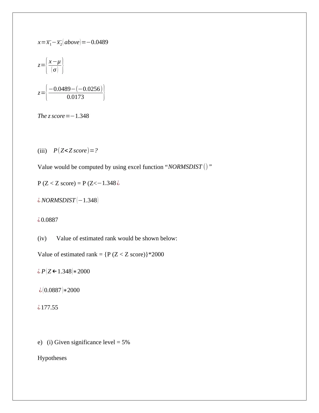
x=x1−x2 ( above ) =−0.0489
z= { x −μ
( σ ) }
z= { −0.0489−(−0.0256)
0.0173 }
The z score=−1.348
(iii) P(Z< Z score)=?
Value would be computed by using excel function “NORMSDIST () ”
P (Z < Z score) = P (Z<−1.348 ¿
¿ NORMSDIST ( −1.348 )
¿ 0.0887
(iv) Value of estimated rank would be shown below:
Value of estimated rank = {P (Z < Z score)}*2000
¿ P ( Z ←1.348 )∗2000
¿ ( 0.0887 )∗2000
¿ 177.55
e) (i) Given significance level = 5%
Hypotheses

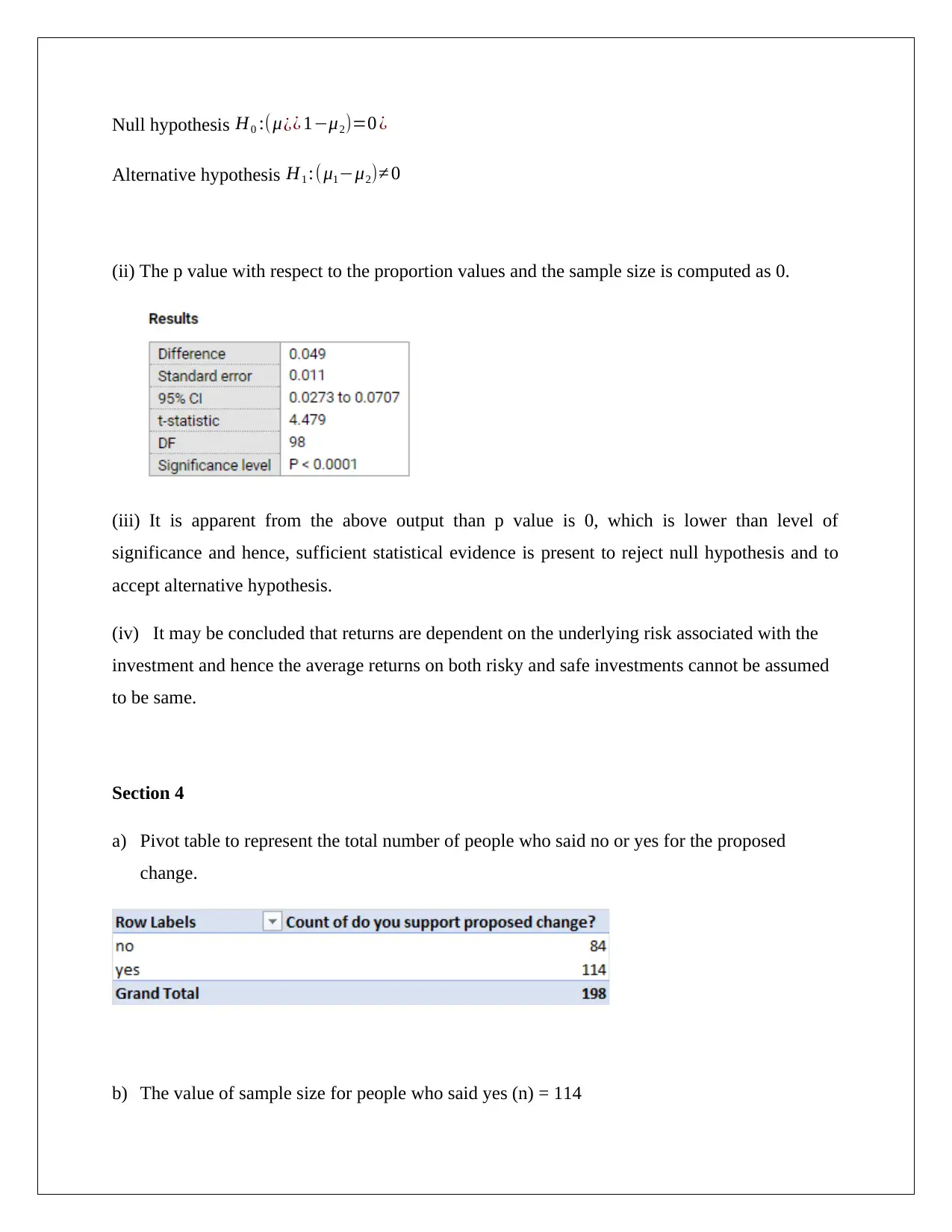
Null hypothesis H0 :(μ¿¿ 1−μ2)=0 ¿
Alternative hypothesis H1 :(μ1−μ2)≠ 0
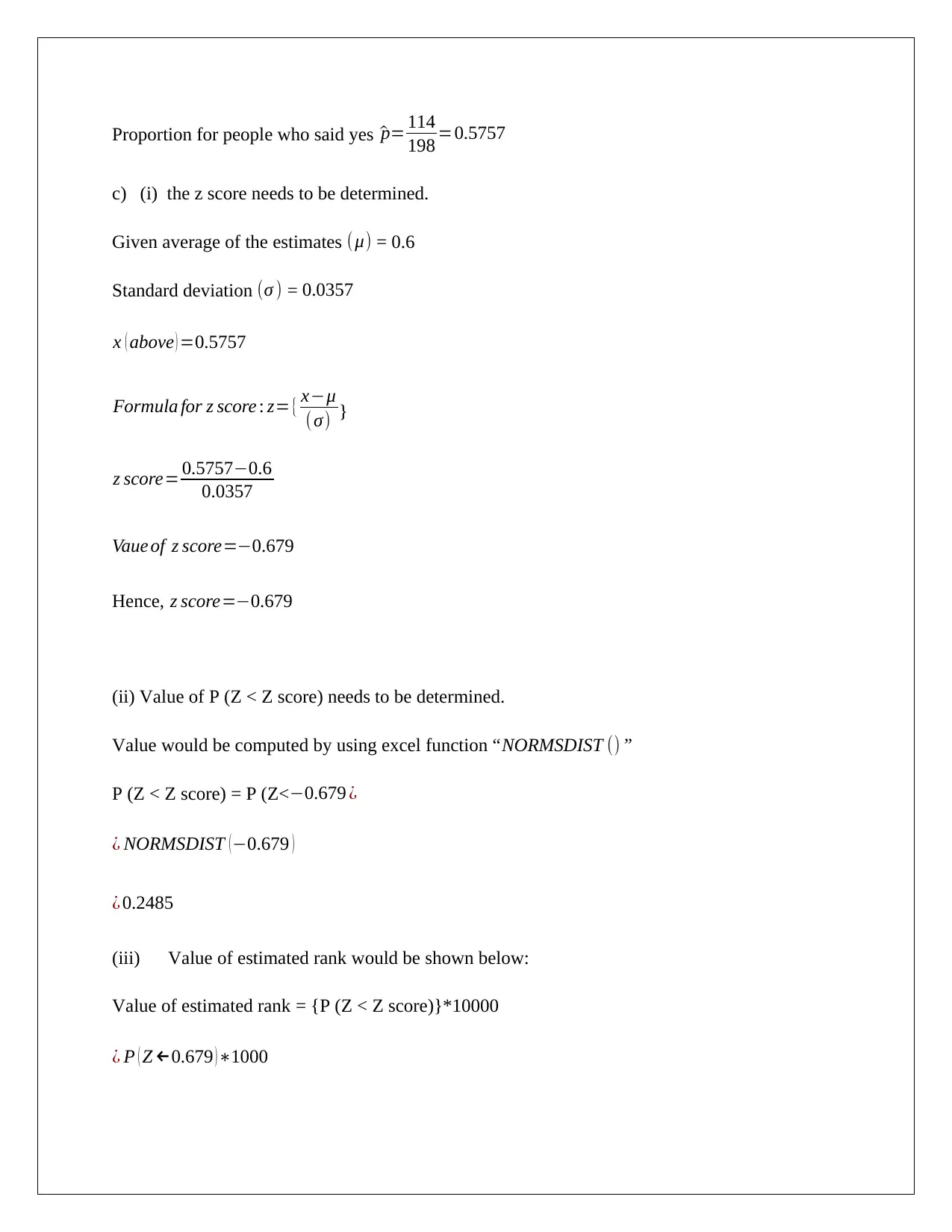
(ii) The p value with respect to the proportion values and the sample size is computed as 0.
(iii) It is apparent from the above output than p value is 0, which is lower than level of
significance and hence, sufficient statistical evidence is present to reject null hypothesis and to
accept alternative hypothesis.
(iv) It may be concluded that returns are dependent on the underlying risk associated with the
investment and hence the average returns on both risky and safe investments cannot be assumed
to be same.
Section 4
a) Pivot table to represent the total number of people who said no or yes for the proposed
change.
b) The value of sample size for people who said yes (n) = 114

Proportion for people who said yes ^p= 114
198 =0.5757
c) (i) the z score needs to be determined.
Given average of the estimates (μ) = 0.6
Standard deviation (σ ) = 0.0357
x ( above ) =0.5757
Formula for z score : z={ x−μ
(σ) }
z score= 0.5757−0.6
0.0357
Vaue of z score=−0.679
Hence, z score=−0.679
(ii) Value of P (Z < Z score) needs to be determined.
Value would be computed by using excel function “NORMSDIST () ”
P (Z < Z score) = P (Z<−0.679 ¿
¿ NORMSDIST (−0.679 )
¿ 0.2485
(iii) Value of estimated rank would be shown below:
Value of estimated rank = {P (Z < Z score)}*10000
¿ P ( Z ←0.679 )∗1000