FINA1108 Project: Evaluating Investment Strategies and Volatility
VerifiedAdded on 2023/01/19
|29
|3173
|50
Project
AI Summary
This project analyzes financial time series data from the FTSE100, focusing on portfolio optimization and volatility modeling. The assignment begins by verifying the stationarity of selected stocks using ACF and PACF tests. It then delves into mean-variance portfolio optimization, including covariance matrix estimation and the construction of an efficient frontier. Furthermore, the project involves forecasting volatility using the GARCH(1,1) model and concludes with an ARMA model analysis. The analysis utilizes data from eight stocks, covering the period from November 2018 to November 2019, to provide a comprehensive understanding of investment strategies and market dynamics. The project aims to provide insights into efficient portfolio construction and volatility forecasting techniques.

PROJECT METHODOLOGIES
Paraphrase This Document
Need a fresh take? Get an instant paraphrase of this document with our AI Paraphraser
TABLE OF CONTENTS
INTRODUCTION...........................................................................................................................1
(A) Evaluation of stationary factor..................................................................................................1
B.......................................................................................................................................................6
(1) Mean variance analysis..........................................................................................................6
(2) Covariance matrix.................................................................................................................7
3 Efficient frontier.......................................................................................................................7
........................................................................................................................................................10
(C) GARCH results........................................................................................................................11
........................................................................................................................................................13
(D) ARMA.....................................................................................................................................20
CONCLUSION..............................................................................................................................22
REFERENCE................................................................................................................................................24
Table 1ASTRAZENECA PACF.....................................................................................................1
Table 2BAE SYSTEMS PACF.......................................................................................................2
Table 3COCA COLA HOLDING AG PACF.................................................................................3
Table 4BRITISH AMERICAN TOBAE SYSTEMSCO PLC PACF.............................................4
Table 5Covariance matrix................................................................................................................7
Table 6Descriptive statistics............................................................................................................7
Table 7Covariance matrix................................................................................................................8
Table 8Target return and average return.........................................................................................9
Table 9Input for efficient frontier....................................................................................................9
Table 10Efficient frontier..............................................................................................................10
Table 15GARCH for ASTRAZENECA 10 months......................................................................11
Table 11ASTRAZENECA regression...........................................................................................11
Table 16Statistics for ASTRAZENECA 10 months.....................................................................12
Table 17GARCH for 2 months......................................................................................................13
Table 13ASTRAZENECA 2 months regression...........................................................................13
Table 18ASTRAZENECA for two months...................................................................................15
Table 19BAE SYSTEMS 10 months............................................................................................16
Table 12BAE SYSTEMSL Regression.........................................................................................16
Table 20Statistics for BAE SYSTEMS 10 months.......................................................................17
Table 21BAE SYSTEMS 2 months..............................................................................................18
Table 14BAE SYSTEMS 2 months regression.............................................................................18
Table 22Statistics for BAE SYSTEMS 2 months.........................................................................20
Table 23ASTRAZENECA regression...........................................................................................20
Table 24BAE SYSTEMS Regression...........................................................................................21
⊘ This is a preview!⊘
Do you want full access?
Subscribe today to unlock all pages.
Trusted by 1+ million students worldwide
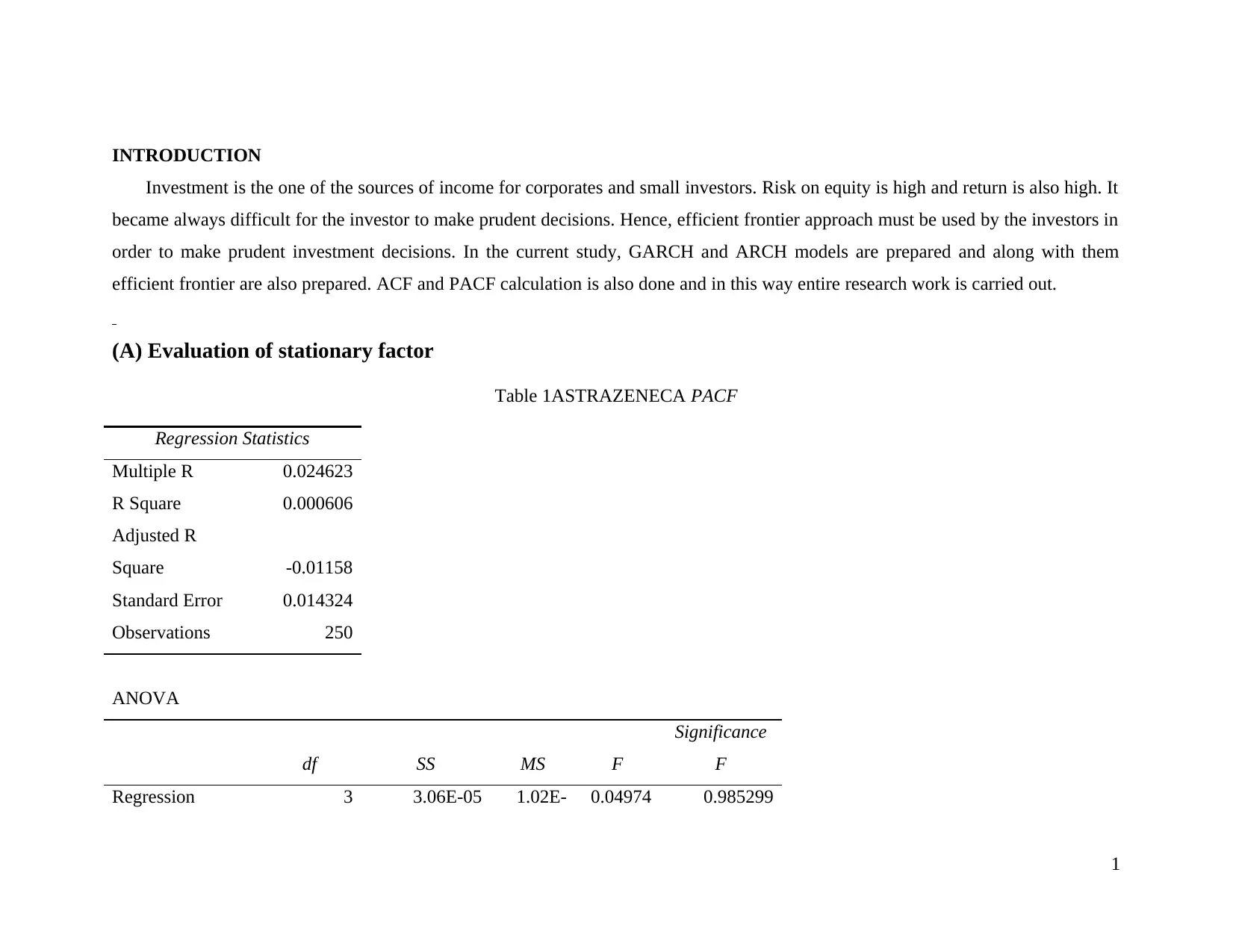
INTRODUCTION
Investment is the one of the sources of income for corporates and small investors. Risk on equity is high and return is also high. It
became always difficult for the investor to make prudent decisions. Hence, efficient frontier approach must be used by the investors in
order to make prudent investment decisions. In the current study, GARCH and ARCH models are prepared and along with them
efficient frontier are also prepared. ACF and PACF calculation is also done and in this way entire research work is carried out.
(A) Evaluation of stationary factor
Table 1ASTRAZENECA PACF
Regression Statistics
Multiple R 0.024623
R Square 0.000606
Adjusted R
Square -0.01158
Standard Error 0.014324
Observations 250
ANOVA
df SS MS F
Significance
F
Regression 3 3.06E-05 1.02E- 0.04974 0.985299
1
Paraphrase This Document
Need a fresh take? Get an instant paraphrase of this document with our AI Paraphraser
05 4
Residual 246 0.050471
0.00020
5
Total 249 0.050502
Coefficient
s
Standard
Error t Stat P-value Lower 95%
Upper
95%
Lower
95.0%
Upper
95.0%
Intercept 0.000596 0.000909
0.65583
8
0.51254
1 -0.00119 0.002386 -0.00119 0.002386
Lag 2 0.023965 0.063764 0.37583
0.70736
7 -0.10163 0.149559 -0.10163 0.149559
Lag 3 -0.00472 0.063757 -0.0741
0.94099
3 -0.1303 0.120855 -0.1303 0.120855
Lag 4 -0.0036 0.062989 -0.05708
0.95453
1 -0.12766 0.120471 -0.12766 0.120471
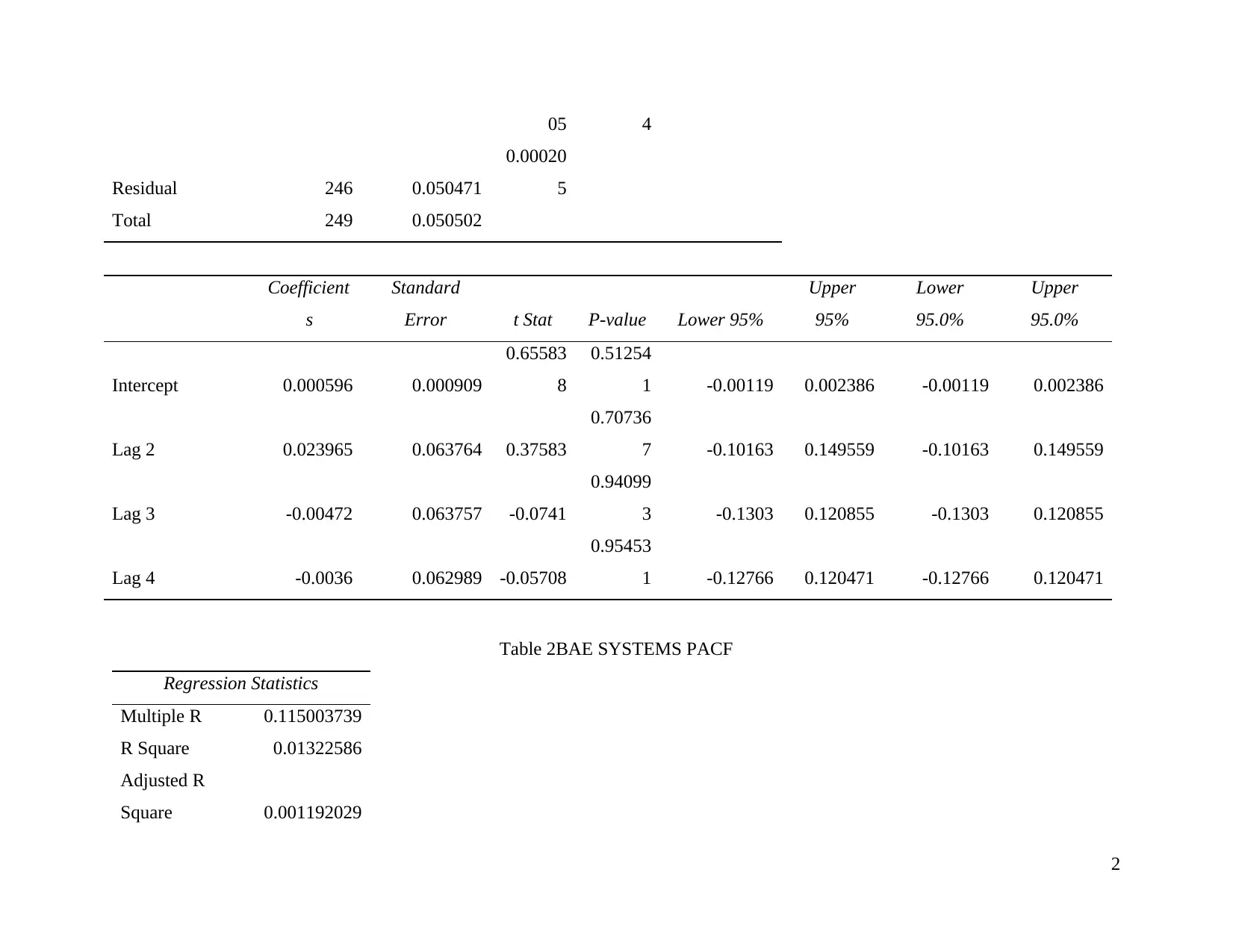
Table 2BAE SYSTEMS PACF
Regression Statistics
Multiple R 0.115003739
R Square 0.01322586
Adjusted R
Square 0.001192029
2
Residual 246 0.050471
0.00020
5
Total 249 0.050502
Coefficient
s
Standard
Error t Stat P-value Lower 95%
Upper
95%
Lower
95.0%
Upper
95.0%
Intercept 0.000596 0.000909
0.65583
8
0.51254
1 -0.00119 0.002386 -0.00119 0.002386
Lag 2 0.023965 0.063764 0.37583
0.70736
7 -0.10163 0.149559 -0.10163 0.149559
Lag 3 -0.00472 0.063757 -0.0741
0.94099
3 -0.1303 0.120855 -0.1303 0.120855
Lag 4 -0.0036 0.062989 -0.05708
0.95453
1 -0.12766 0.120471 -0.12766 0.120471
Table 2BAE SYSTEMS PACF
Regression Statistics
Multiple R 0.115003739
R Square 0.01322586
Adjusted R
Square 0.001192029
2
Standard Error 0.014060995
Observations 250
ANOVA
df SS MS F
Significance
F
Regression 3 0.000652 0.000217 1.099056 0.350169
Residual 246 0.048637 0.000198
Total 249 0.049289
Coefficients
Standard
Error t Stat P-value Lower 95%
Upper
95%
Lower
95.0%
Upper
95.0%
Intercept 0.000380909 0.00089 0.427991 0.669032 -0.00137 0.002134 -0.00137 0.002134
Lag 2 0.113199299 0.063782 1.774779 0.077171 -0.01243 0.238828 -0.01243 0.238828
Lag 3 0.007945121 0.064332 0.123502 0.901811 -0.11877 0.134657 -0.11877 0.134657
Lag 4
-
0.017024478 0.064132 -0.26546 0.790876 -0.14334 0.109293 -0.14334 0.109293
Table 3COCA COLA HOLDING AG PACF
Regression Statistics
Multiple R 0.183819
3
⊘ This is a preview!⊘
Do you want full access?
Subscribe today to unlock all pages.
Trusted by 1+ million students worldwide
R Square 0.03379
Adjusted R
Square 0.022006
Standard Error 0.015573
Observations 250
ANOVA
df SS MS F
Significance
F
Regression 3 0.002086 0.000695 2.867637 0.037184
Residual 246 0.05966 0.000243
Total 249 0.061746
Coefficients
Standard
Error t Stat P-value Lower 95%
Upper
95%
Lower
95.0%
Upper
95.0%
Intercept -1.5E-05 0.000985 -0.01552 0.987632 -0.00196 0.001925 -0.00196 0.001925
Lag 2 -0.14893 0.063662 -2.33935 0.020118 -0.27432 -0.02354 -0.27432 -0.02354
Lag 3 -0.13129 0.063893 -2.05479 0.040956 -0.25713 -0.00544 -0.25713 -0.00544
Lag 4 -0.05105 0.062434 -0.81772 0.414306 -0.17403 0.07192 -0.17403 0.07192
4
Paraphrase This Document
Need a fresh take? Get an instant paraphrase of this document with our AI Paraphraser
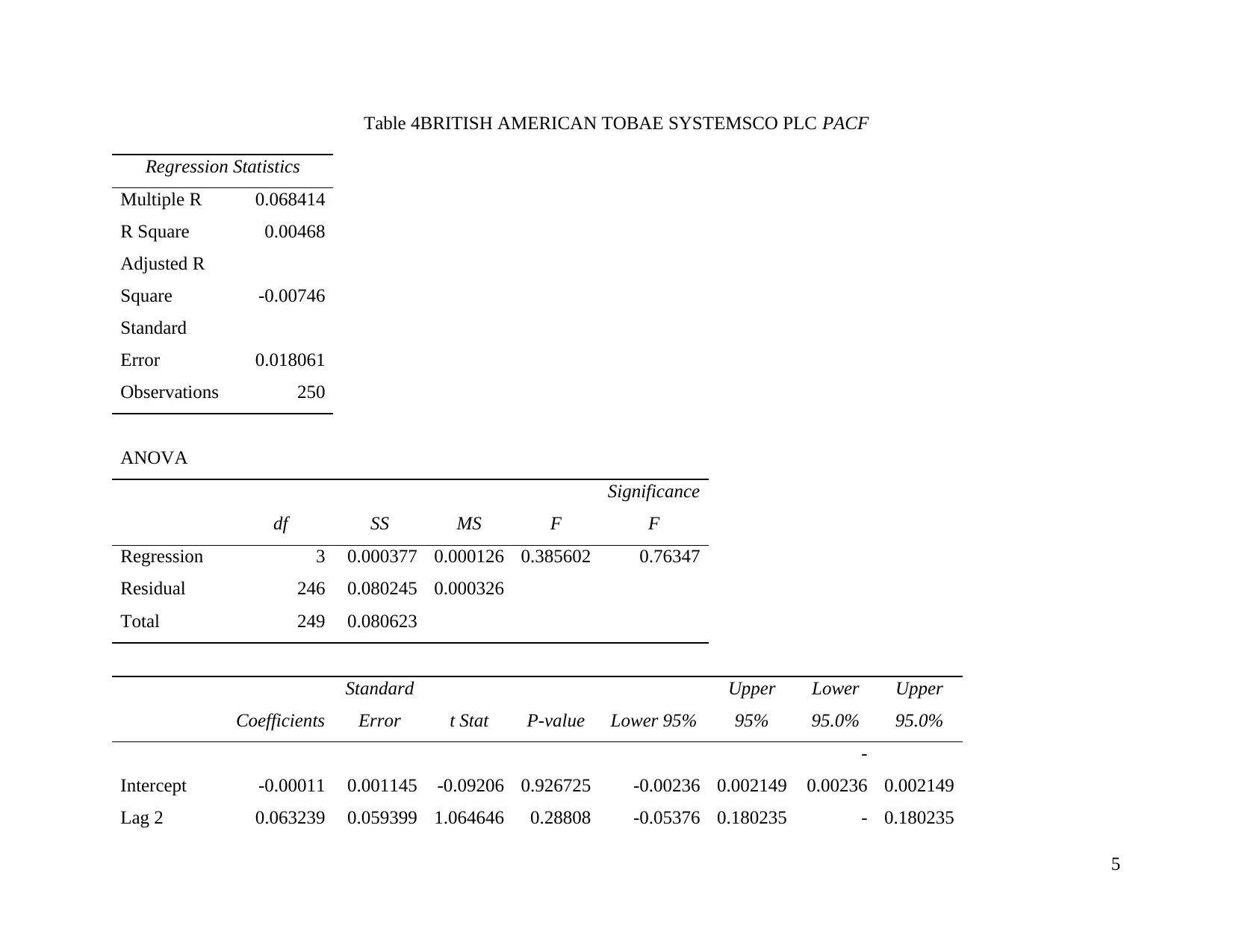
Table 4BRITISH AMERICAN TOBAE SYSTEMSCO PLC PACF
Regression Statistics
Multiple R 0.068414
R Square 0.00468
Adjusted R
Square -0.00746
Standard
Error 0.018061
Observations 250
ANOVA
df SS MS F
Significance
F
Regression 3 0.000377 0.000126 0.385602 0.76347
Residual 246 0.080245 0.000326
Total 249 0.080623
Coefficients
Standard
Error t Stat P-value Lower 95%
Upper
95%
Lower
95.0%
Upper
95.0%
Intercept -0.00011 0.001145 -0.09206 0.926725 -0.00236 0.002149
-
0.00236 0.002149
Lag 2 0.063239 0.059399 1.064646 0.28808 -0.05376 0.180235 - 0.180235
5
0.05376
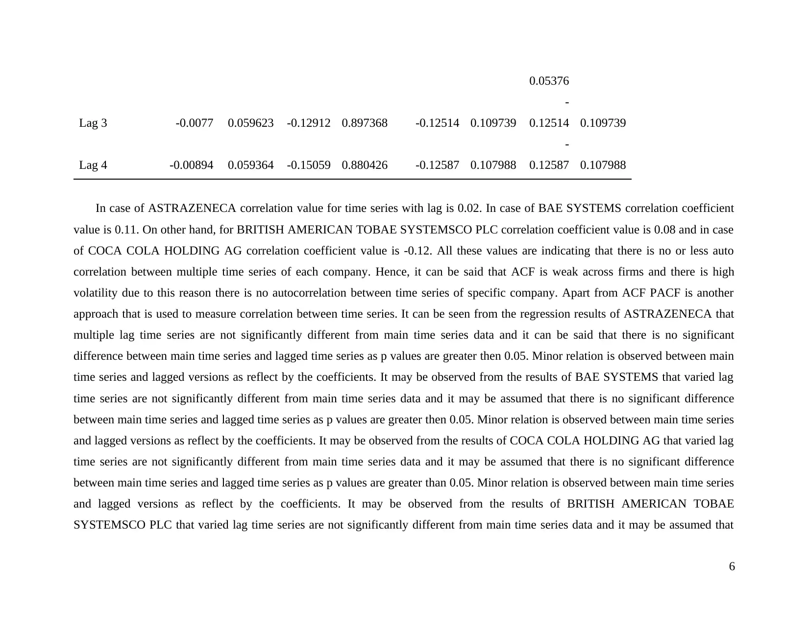
Lag 3 -0.0077 0.059623 -0.12912 0.897368 -0.12514 0.109739
-
0.12514 0.109739
Lag 4 -0.00894 0.059364 -0.15059 0.880426 -0.12587 0.107988
-
0.12587 0.107988
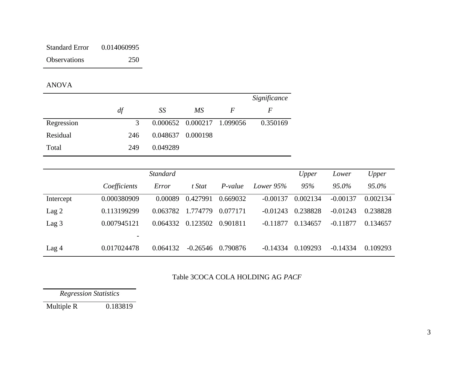
In case of ASTRAZENECA correlation value for time series with lag is 0.02. In case of BAE SYSTEMS correlation coefficient
value is 0.11. On other hand, for BRITISH AMERICAN TOBAE SYSTEMSCO PLC correlation coefficient value is 0.08 and in case
of COCA COLA HOLDING AG correlation coefficient value is -0.12. All these values are indicating that there is no or less auto
correlation between multiple time series of each company. Hence, it can be said that ACF is weak across firms and there is high
volatility due to this reason there is no autocorrelation between time series of specific company. Apart from ACF PACF is another
approach that is used to measure correlation between time series. It can be seen from the regression results of ASTRAZENECA that
multiple lag time series are not significantly different from main time series data and it can be said that there is no significant
difference between main time series and lagged time series as p values are greater then 0.05. Minor relation is observed between main
time series and lagged versions as reflect by the coefficients. It may be observed from the results of BAE SYSTEMS that varied lag
time series are not significantly different from main time series data and it may be assumed that there is no significant difference
between main time series and lagged time series as p values are greater then 0.05. Minor relation is observed between main time series
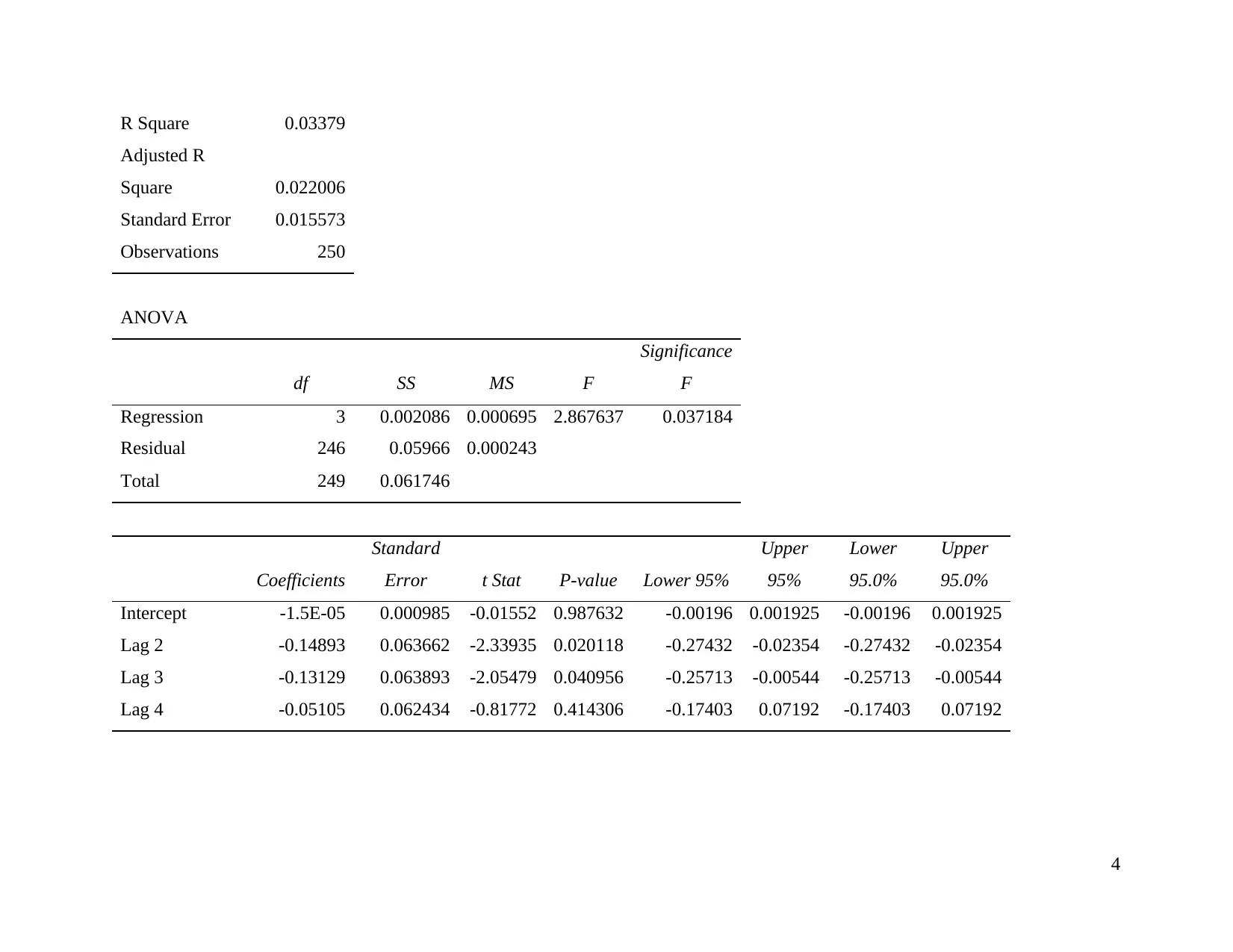
and lagged versions as reflect by the coefficients. It may be observed from the results of COCA COLA HOLDING AG that varied lag
time series are not significantly different from main time series data and it may be assumed that there is no significant difference
between main time series and lagged time series as p values are greater than 0.05. Minor relation is observed between main time series
and lagged versions as reflect by the coefficients. It may be observed from the results of BRITISH AMERICAN TOBAE
SYSTEMSCO PLC that varied lag time series are not significantly different from main time series data and it may be assumed that
6
Lag 3 -0.0077 0.059623 -0.12912 0.897368 -0.12514 0.109739
-
0.12514 0.109739
Lag 4 -0.00894 0.059364 -0.15059 0.880426 -0.12587 0.107988
-
0.12587 0.107988
In case of ASTRAZENECA correlation value for time series with lag is 0.02. In case of BAE SYSTEMS correlation coefficient
value is 0.11. On other hand, for BRITISH AMERICAN TOBAE SYSTEMSCO PLC correlation coefficient value is 0.08 and in case
of COCA COLA HOLDING AG correlation coefficient value is -0.12. All these values are indicating that there is no or less auto
correlation between multiple time series of each company. Hence, it can be said that ACF is weak across firms and there is high
volatility due to this reason there is no autocorrelation between time series of specific company. Apart from ACF PACF is another
approach that is used to measure correlation between time series. It can be seen from the regression results of ASTRAZENECA that
multiple lag time series are not significantly different from main time series data and it can be said that there is no significant
difference between main time series and lagged time series as p values are greater then 0.05. Minor relation is observed between main
time series and lagged versions as reflect by the coefficients. It may be observed from the results of BAE SYSTEMS that varied lag
time series are not significantly different from main time series data and it may be assumed that there is no significant difference
between main time series and lagged time series as p values are greater then 0.05. Minor relation is observed between main time series
and lagged versions as reflect by the coefficients. It may be observed from the results of COCA COLA HOLDING AG that varied lag
time series are not significantly different from main time series data and it may be assumed that there is no significant difference
between main time series and lagged time series as p values are greater than 0.05. Minor relation is observed between main time series
and lagged versions as reflect by the coefficients. It may be observed from the results of BRITISH AMERICAN TOBAE
SYSTEMSCO PLC that varied lag time series are not significantly different from main time series data and it may be assumed that
6
⊘ This is a preview!⊘
Do you want full access?
Subscribe today to unlock all pages.
Trusted by 1+ million students worldwide
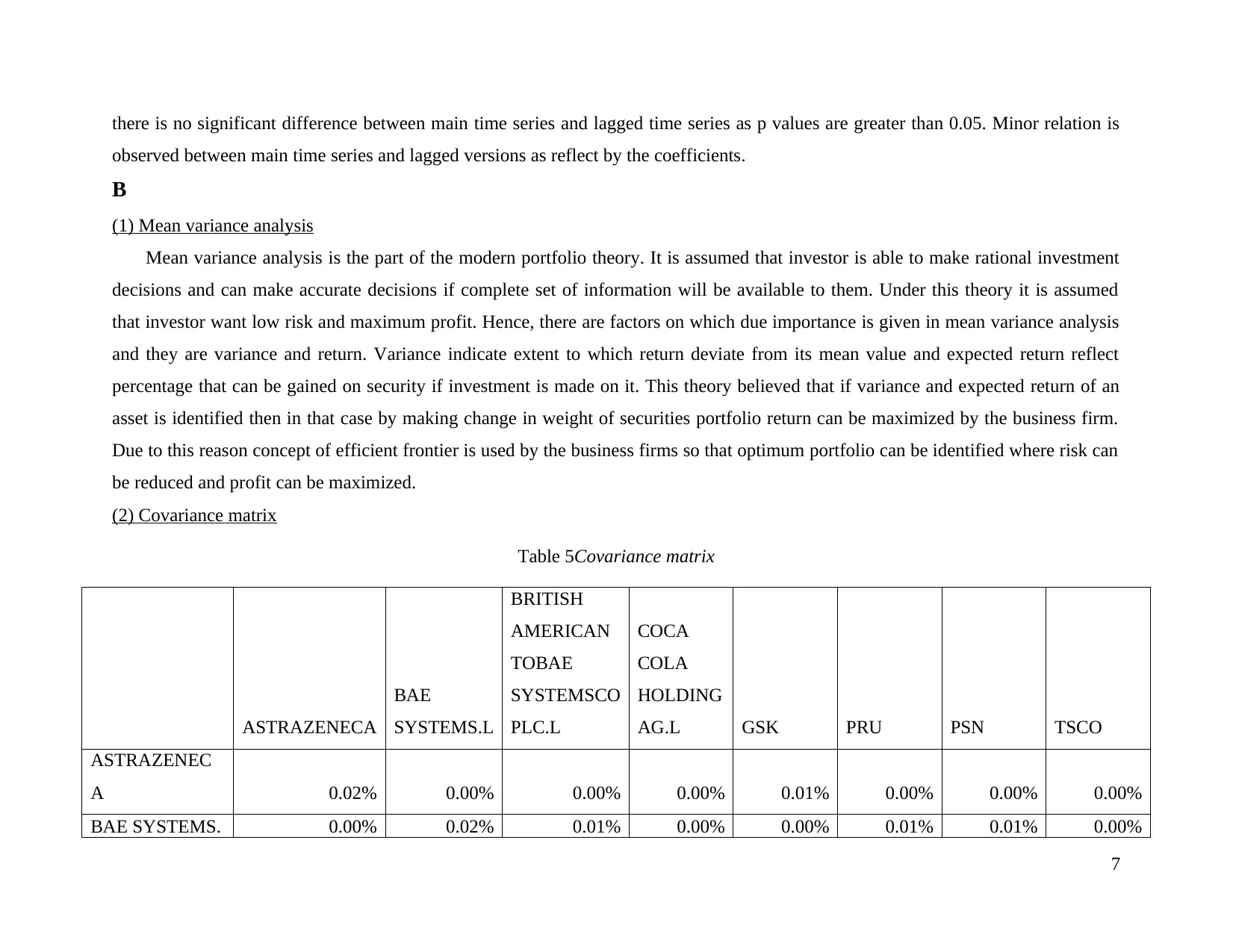
there is no significant difference between main time series and lagged time series as p values are greater than 0.05. Minor relation is
observed between main time series and lagged versions as reflect by the coefficients.
B
(1) Mean variance analysis
Mean variance analysis is the part of the modern portfolio theory. It is assumed that investor is able to make rational investment
decisions and can make accurate decisions if complete set of information will be available to them. Under this theory it is assumed
that investor want low risk and maximum profit. Hence, there are factors on which due importance is given in mean variance analysis
and they are variance and return. Variance indicate extent to which return deviate from its mean value and expected return reflect
percentage that can be gained on security if investment is made on it. This theory believed that if variance and expected return of an
asset is identified then in that case by making change in weight of securities portfolio return can be maximized by the business firm.
Due to this reason concept of efficient frontier is used by the business firms so that optimum portfolio can be identified where risk can
be reduced and profit can be maximized.
(2) Covariance matrix
Table 5Covariance matrix
ASTRAZENECA
BAE
SYSTEMS.L
BRITISH
AMERICAN
TOBAE
SYSTEMSCO
PLC.L
COCA
COLA
HOLDING
AG.L GSK PRU PSN TSCO
ASTRAZENEC
A 0.02% 0.00% 0.00% 0.00% 0.01% 0.00% 0.00% 0.00%
BAE SYSTEMS. 0.00% 0.02% 0.01% 0.00% 0.00% 0.01% 0.01% 0.00%
7
Paraphrase This Document
Need a fresh take? Get an instant paraphrase of this document with our AI Paraphraser
L
BRITISH
AMERICAN
TOBAE
SYSTEMSCO
PLC.L 0.00% 0.01% 0.04% 0.01% 0.00% 0.01% 0.00% 0.00%
COCA COLA
HOLDING AG.L 0.00% 0.00% 0.01% 0.03% 0.00% 0.01% 0.00% 0.00%
GSK 0.01% 0.00% 0.00% 0.00% 0.01% 0.00% 0.00% 0.00%
PRU 0.00% 0.01% 0.01% 0.01% 0.00% 0.03% 0.01% 0.01%
PSN 0.00% 0.01% 0.00% 0.00% 0.00% 0.01% 0.04% 0.01%
TSCO 0.00% 0.00% 0.00% 0.00% 0.00% 0.01% 0.01% 0.02%
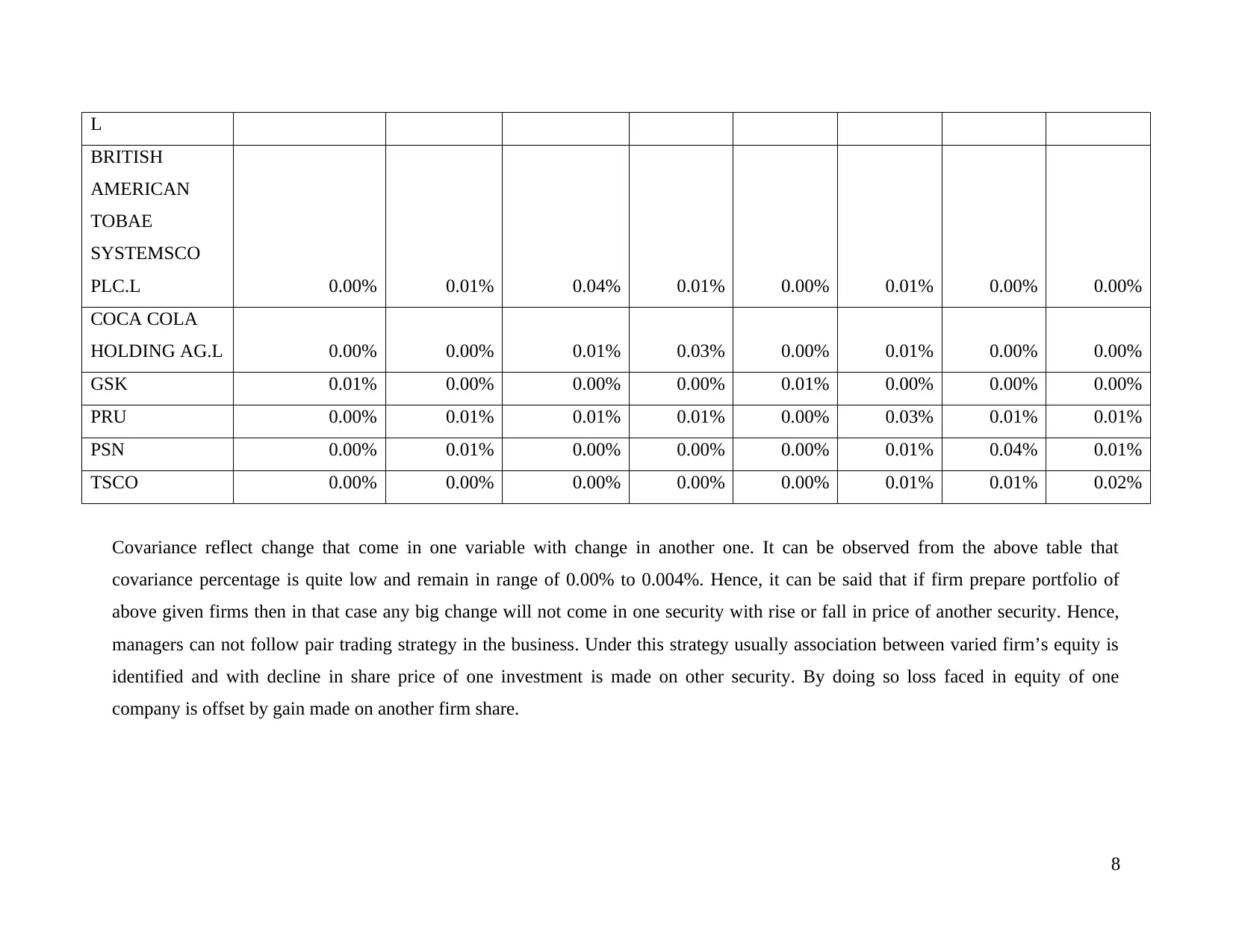
Covariance reflect change that come in one variable with change in another one. It can be observed from the above table that
covariance percentage is quite low and remain in range of 0.00% to 0.004%. Hence, it can be said that if firm prepare portfolio of
above given firms then in that case any big change will not come in one security with rise or fall in price of another security. Hence,
managers can not follow pair trading strategy in the business. Under this strategy usually association between varied firm’s equity is
identified and with decline in share price of one investment is made on other security. By doing so loss faced in equity of one
company is offset by gain made on another firm share.
8
BRITISH
AMERICAN
TOBAE
SYSTEMSCO
PLC.L 0.00% 0.01% 0.04% 0.01% 0.00% 0.01% 0.00% 0.00%
COCA COLA
HOLDING AG.L 0.00% 0.00% 0.01% 0.03% 0.00% 0.01% 0.00% 0.00%
GSK 0.01% 0.00% 0.00% 0.00% 0.01% 0.00% 0.00% 0.00%
PRU 0.00% 0.01% 0.01% 0.01% 0.00% 0.03% 0.01% 0.01%
PSN 0.00% 0.01% 0.00% 0.00% 0.00% 0.01% 0.04% 0.01%
TSCO 0.00% 0.00% 0.00% 0.00% 0.00% 0.01% 0.01% 0.02%
Covariance reflect change that come in one variable with change in another one. It can be observed from the above table that
covariance percentage is quite low and remain in range of 0.00% to 0.004%. Hence, it can be said that if firm prepare portfolio of
above given firms then in that case any big change will not come in one security with rise or fall in price of another security. Hence,
managers can not follow pair trading strategy in the business. Under this strategy usually association between varied firm’s equity is
identified and with decline in share price of one investment is made on other security. By doing so loss faced in equity of one
company is offset by gain made on another firm share.
8
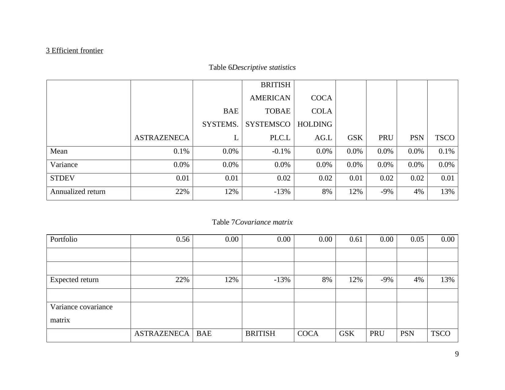
3 Efficient frontier
Table 6Descriptive statistics
ASTRAZENECA
BAE
SYSTEMS.
L
BRITISH
AMERICAN
TOBAE
SYSTEMSCO
PLC.L
COCA
COLA
HOLDING
AG.L GSK PRU PSN TSCO
Mean 0.1% 0.0% -0.1% 0.0% 0.0% 0.0% 0.0% 0.1%
Variance 0.0% 0.0% 0.0% 0.0% 0.0% 0.0% 0.0% 0.0%
STDEV 0.01 0.01 0.02 0.02 0.01 0.02 0.02 0.01
Annualized return 22% 12% -13% 8% 12% -9% 4% 13%
Table 7Covariance matrix
Portfolio 0.56 0.00 0.00 0.00 0.61 0.00 0.05 0.00
Expected return 22% 12% -13% 8% 12% -9% 4% 13%
Variance covariance
matrix
ASTRAZENECA BAE BRITISH COCA GSK PRU PSN TSCO
9
⊘ This is a preview!⊘
Do you want full access?
Subscribe today to unlock all pages.
Trusted by 1+ million students worldwide
1 out of 29
Related Documents


Your All-in-One AI-Powered Toolkit for Academic Success.
+13062052269
info@desklib.com
Available 24*7 on WhatsApp / Email
![[object Object]](/_next/static/media/star-bottom.7253800d.svg)
Unlock your academic potential
Copyright © 2020–2026 A2Z Services. All Rights Reserved. Developed and managed by ZUCOL.