Financial Modelling Project: University Financial Analysis Report

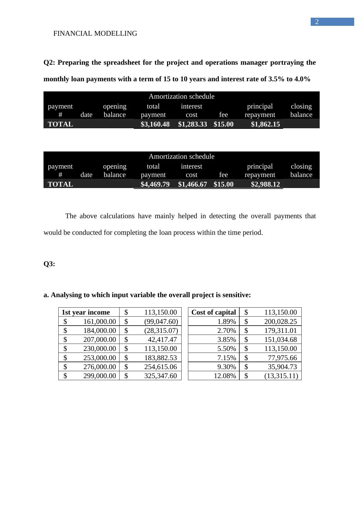
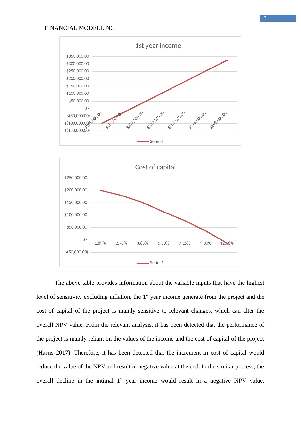
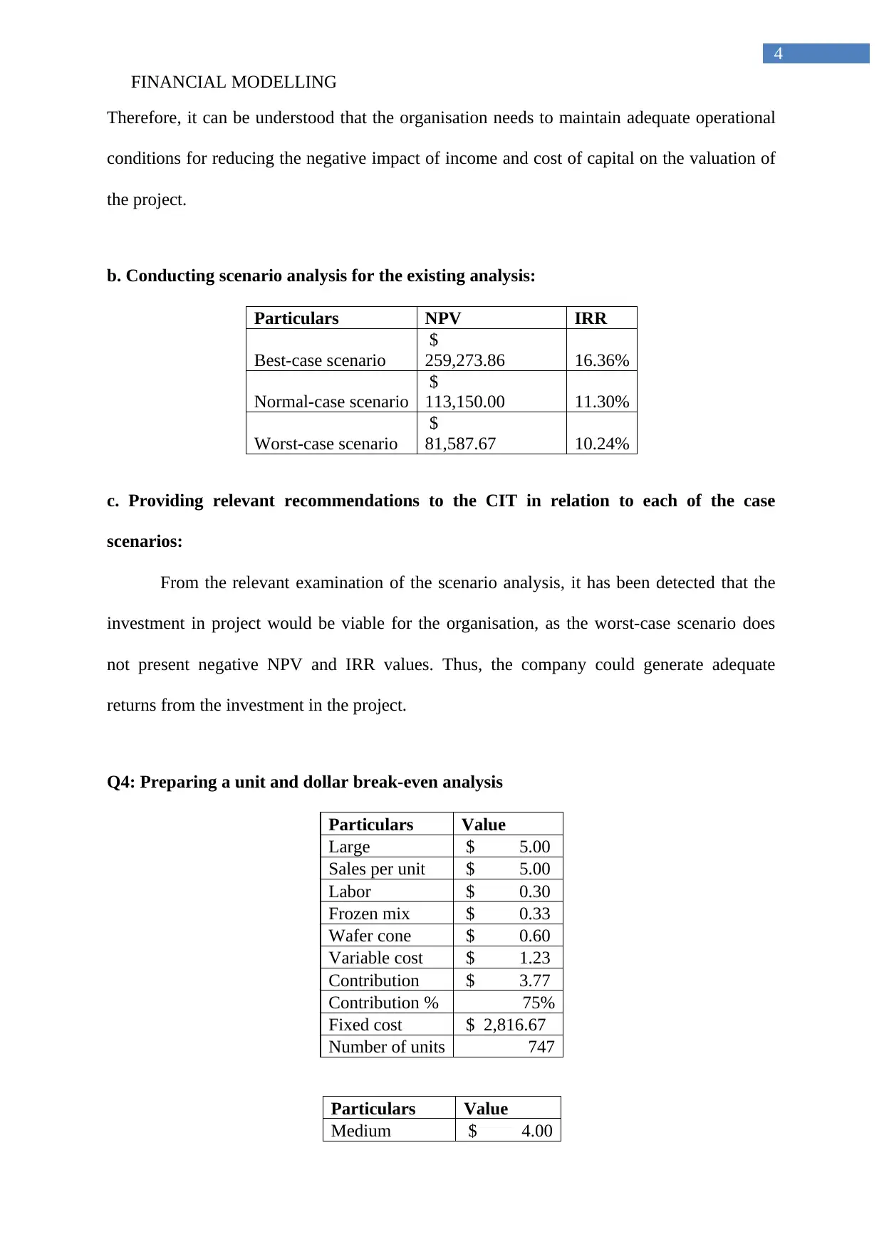
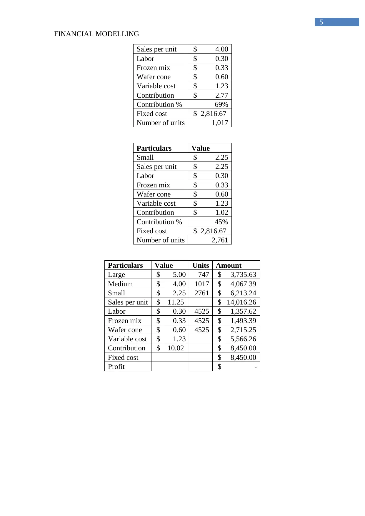
This financial modeling project delves into key financial concepts. It begins with preparing a spreadsheet to portray monthly loan payments with varying terms and interest rates, constructing an amortization schedule. The project then proceeds to analyze the sensitivity of a project to different inpu...Read More

Running head: FINANCIAL MODELLING
Financial Modelling
Name of the Student:
Name of the University:
Authors Note:

FINANCIAL MODELLING
1
Table of Contents
Q2: Preparing the spreadsheet for the project and operations manager portraying the monthly
loan payments with a term of 15 to 10 years and interest rate of 3.5% to 4.0%........................2
Q3:..............................................................................................................................................2
a. Analysing to which input variable the overall project is sensitive:........................................2
b. Conducting scenario analysis for the existing analysis:.........................................................4
c. Providing relevant recommendations to the CIT in relation to each of the case scenarios:...4
Q4: Preparing a unit and dollar break-even analysis.................................................................4
Reference:..................................................................................................................................6

FINANCIAL MODELLING
2
Q2: Preparing the spreadsheet for the project and operations manager portraying the
monthly loan payments with a term of 15 to 10 years and interest rate of 3.5% to 4.0%
Amortization schedule
payment
# date
opening
balance
total
payment
interest
cost fee
principal
repayment
closing
balance
TOTAL $3,160.48 $1,283.33 $15.00 $1,862.15
Amortization schedule
payment
# date
opening
balance
total
payment
interest
cost fee
principal
repayment
closing
balance
TOTAL $4,469.79 $1,466.67 $15.00 $2,988.12
The above calculations have mainly helped in detecting the overall payments that
would be conducted for completing the loan process within the time period.
Q3:
a. Analysing to which input variable the overall project is sensitive:
1st year income $ 113,150.00 Cost of capital $ 113,150.00
$ 161,000.00 $ (99,047.60) 1.89% $ 200,028.25
$ 184,000.00 $ (28,315.07) 2.70% $ 179,311.01
$ 207,000.00 $ 42,417.47 3.85% $ 151,034.68
$ 230,000.00 $ 113,150.00 5.50% $ 113,150.00
$ 253,000.00 $ 183,882.53 7.15% $ 77,975.66
$ 276,000.00 $ 254,615.06 9.30% $ 35,904.73
$ 299,000.00 $ 325,347.60 12.08% $ (13,315.11)

FINANCIAL MODELLING
3
$161,000.00
$184,000.00
$207,000.00
$230,000.00
$253,000.00
$276,000.00
$299,000.00
$(150,000.00)
$(100,000.00)
$(50,000.00)
$-
$50,000.00
$100,000.00
$150,000.00
$200,000.00
$250,000.00
$300,000.00
$350,000.00
1st year income
Series1
1.89% 2.70% 3.85% 5.50% 7.15% 9.30% 12.08%
$(50,000.00)
$-
$50,000.00
$100,000.00
$150,000.00
$200,000.00
$250,000.00
Cost of capital
Series1
The above table provides information about the variable inputs that have the highest
level of sensitivity excluding inflation, the 1st year income generate from the project and the
cost of capital of the project is mainly sensitive to relevant changes, which can alter the
overall NPV value. From the relevant analysis, it has been detected that the performance of
the project is mainly reliant on the values of the income and the cost of capital of the project
(Harris 2017). Therefore, it has been detected that the increment in cost of capital would
reduce the value of the NPV and result in negative value at the end. In the similar process, the
overall decline in the intimal 1st year income would result in a negative NPV value.

FINANCIAL MODELLING
4
Therefore, it can be understood that the organisation needs to maintain adequate operational
conditions for reducing the negative impact of income and cost of capital on the valuation of
the project.
b. Conducting scenario analysis for the existing analysis:
Particulars NPV IRR
Best-case scenario
$
259,273.86 16.36%
Normal-case scenario
$
113,150.00 11.30%
Worst-case scenario
$
81,587.67 10.24%
c. Providing relevant recommendations to the CIT in relation to each of the case
scenarios:
From the relevant examination of the scenario analysis, it has been detected that the
investment in project would be viable for the organisation, as the worst-case scenario does
not present negative NPV and IRR values. Thus, the company could generate adequate
returns from the investment in the project.
Q4: Preparing a unit and dollar break-even analysis
Particulars Value
Large $ 5.00
Sales per unit $ 5.00
Labor $ 0.30
Frozen mix $ 0.33
Wafer cone $ 0.60
Variable cost $ 1.23
Contribution $ 3.77
Contribution % 75%
Fixed cost $ 2,816.67
Number of units 747
Particulars Value
Medium $ 4.00

FINANCIAL MODELLING
5
Sales per unit $ 4.00
Labor $ 0.30
Frozen mix $ 0.33
Wafer cone $ 0.60
Variable cost $ 1.23
Contribution $ 2.77
Contribution % 69%
Fixed cost $ 2,816.67
Number of units 1,017
Particulars Value
Small $ 2.25
Sales per unit $ 2.25
Labor $ 0.30
Frozen mix $ 0.33
Wafer cone $ 0.60
Variable cost $ 1.23
Contribution $ 1.02
Contribution % 45%
Fixed cost $ 2,816.67
Number of units 2,761
Particulars Value Units Amount
Large $ 5.00 747 $ 3,735.63
Medium $ 4.00 1017 $ 4,067.39
Small $ 2.25 2761 $ 6,213.24
Sales per unit $ 11.25 $ 14,016.26
Labor $ 0.30 4525 $ 1,357.62
Frozen mix $ 0.33 4525 $ 1,493.39
Wafer cone $ 0.60 4525 $ 2,715.25
Variable cost $ 1.23 $ 5,566.26
Contribution $ 10.02 $ 8,450.00
Fixed cost $ 8,450.00
Profit $ -

FINANCIAL MODELLING
6
Reference:
Harris, E., 2017. Strategic project risk appraisal and management. Routledge.