Financial Economics Project: Portfolio Analysis and Efficient Frontier

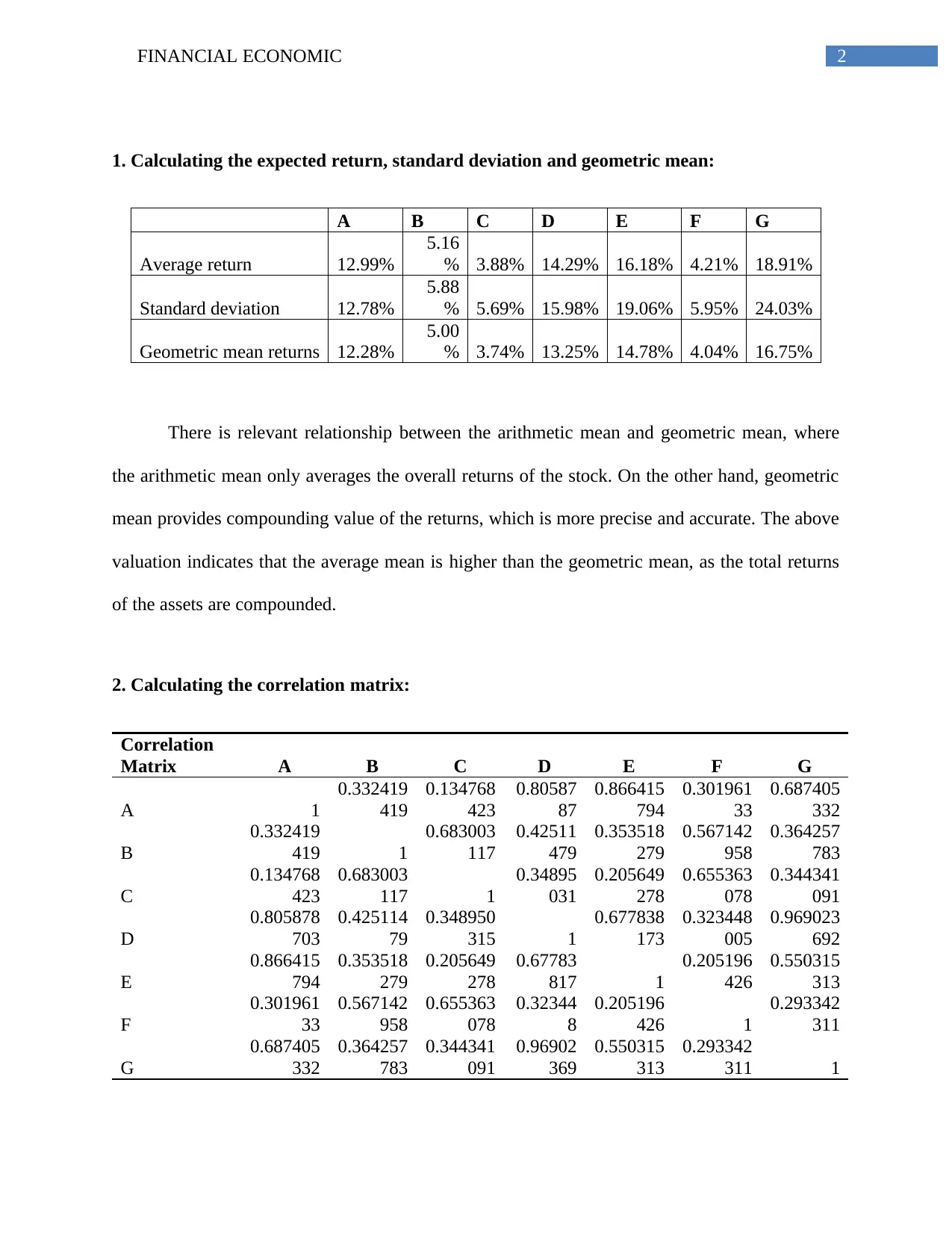
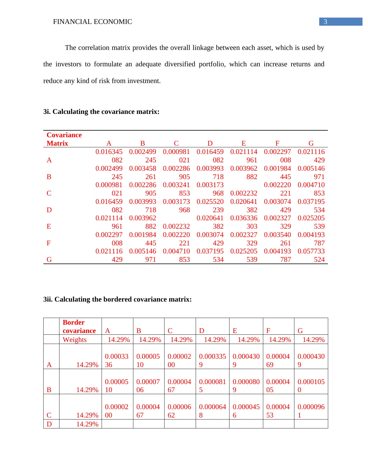
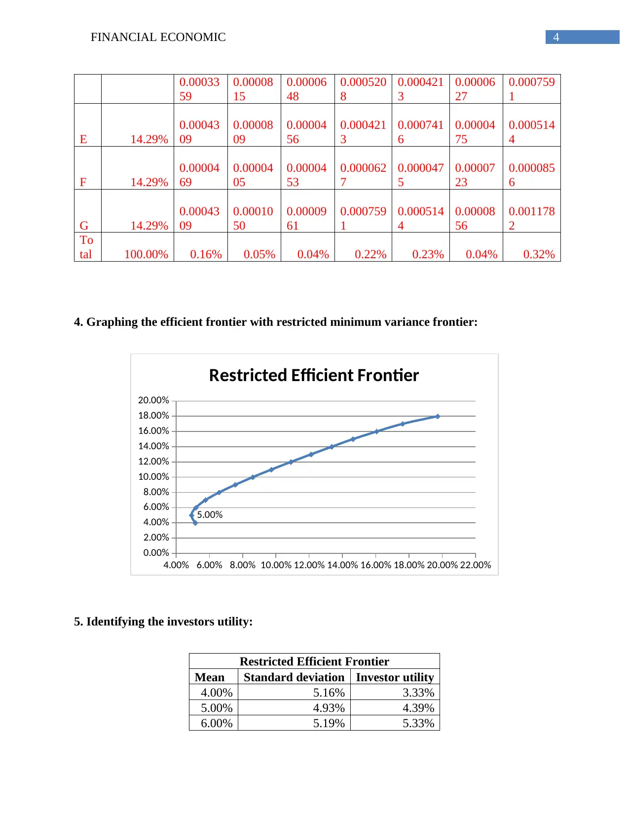
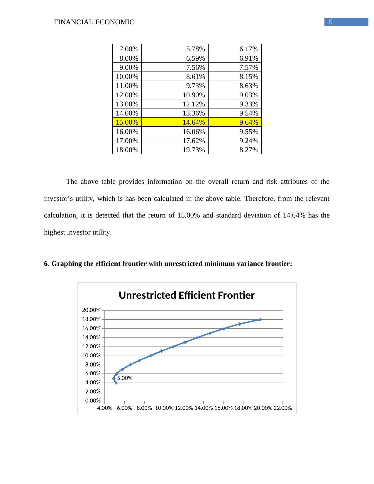
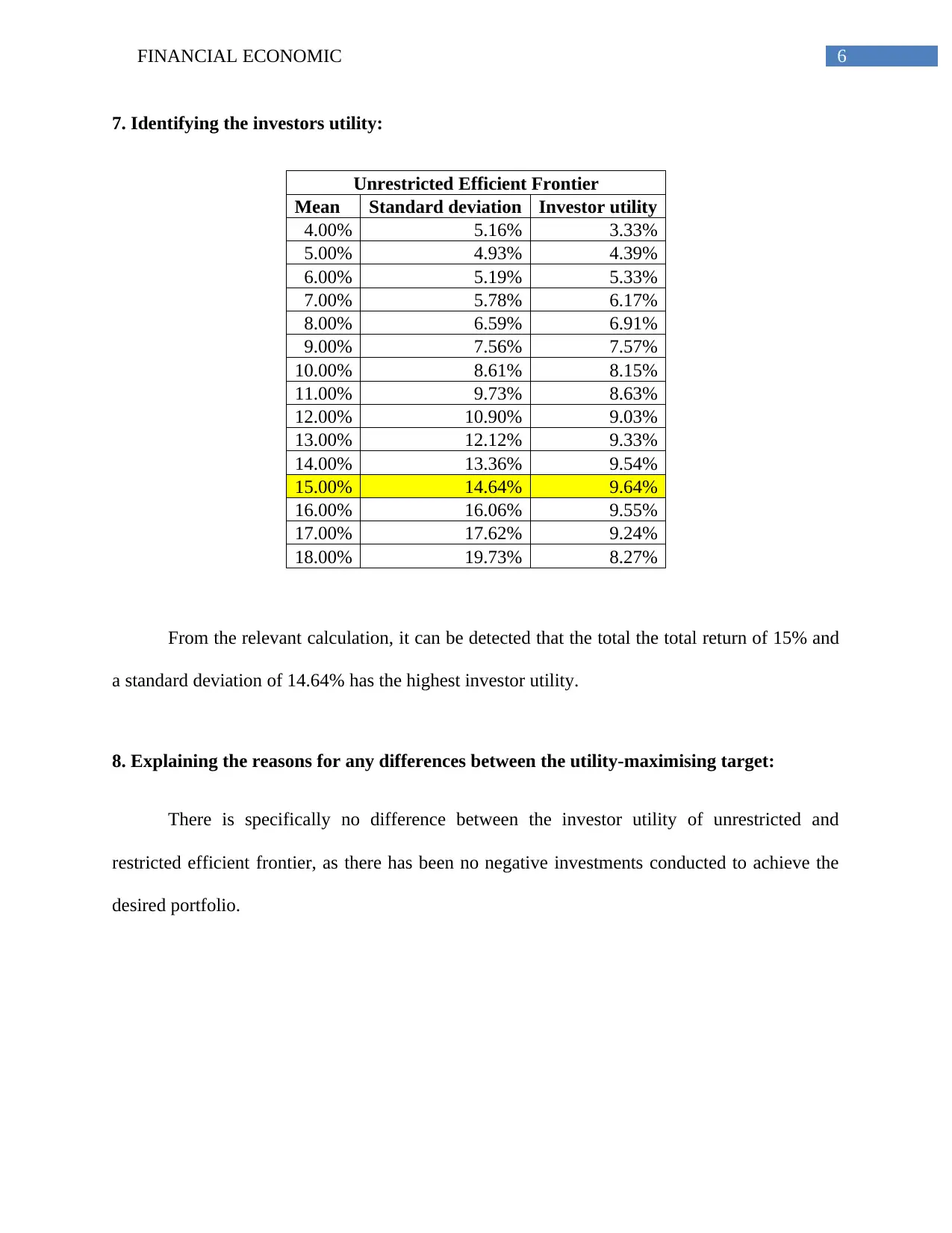
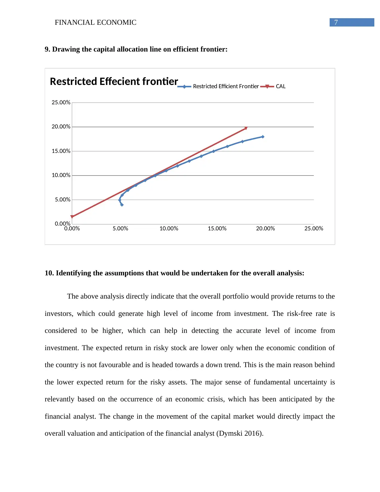
This financial economics project undertakes a comprehensive analysis of portfolio optimization. It begins by calculating the expected return, standard deviation, and geometric mean for various assets. The project then proceeds to compute the correlation and covariance matrices, providing insights into the relationships between different assets. Utilizing these calculations, the project graphs both restricted and unrestricted efficient frontiers, demonstrating the trade-off between risk and return. Investor utility is identified for different points on the efficient frontier. The project also draws the capital allocation line to illustrate the optimal allocation of capital. Finally, the analysis identifies the assumptions underlying the entire process and provides a detailed explanation of the factors influencing investor utility maximization and identifies the differences between the utility-maximizing targets. The project incorporates relevant references to support its findings.

Running head: FINANCIAL ECONOMIC
Financial Economic
Name of the Student:
Name of the University:
Author’s Note:
Course ID:

1FINANCIAL ECONOMIC
Table of Contents
1. Calculating the expected return, standard deviation and geometric mean:.................................2
2. Calculating the correlation matrix:..............................................................................................2
3i. Calculating the covariance matrix:.............................................................................................3
3ii. Calculating the bordered covariance matrix:.............................................................................3
4. Graphing the efficient frontier with restricted minimum variance frontier:................................4
5. Identifying the investors utility:...................................................................................................4
6. Graphing the efficient frontier with unrestricted minimum variance frontier:............................5
7. Identifying the investors utility:...................................................................................................6
8. Explaining the reasons for any differences between the utility-maximising target:...................6
9. Drawing the capital allocation line on efficient frontier:.............................................................7
10. Identifying the assumptions that would be undertaken for the overall analysis:.......................7
References and Bibliography:..........................................................................................................9

2FINANCIAL ECONOMIC
1. Calculating the expected return, standard deviation and geometric mean:
A B C D E F G
Average return 12.99%
5.16
% 3.88% 14.29% 16.18% 4.21% 18.91%
Standard deviation 12.78%
5.88
% 5.69% 15.98% 19.06% 5.95% 24.03%
Geometric mean returns 12.28%
5.00
% 3.74% 13.25% 14.78% 4.04% 16.75%
There is relevant relationship between the arithmetic mean and geometric mean, where
the arithmetic mean only averages the overall returns of the stock. On the other hand, geometric
mean provides compounding value of the returns, which is more precise and accurate. The above
valuation indicates that the average mean is higher than the geometric mean, as the total returns
of the assets are compounded.
2. Calculating the correlation matrix:
Correlation
Matrix A B C D E F G
A 1
0.332419
419
0.134768
423
0.80587
87
0.866415
794
0.301961
33
0.687405
332
B
0.332419
419 1
0.683003
117
0.42511
479
0.353518
279
0.567142
958
0.364257
783
C
0.134768
423
0.683003
117 1
0.34895
031
0.205649
278
0.655363
078
0.344341
091
D
0.805878
703
0.425114
79
0.348950
315 1
0.677838
173
0.323448
005
0.969023
692
E
0.866415
794
0.353518
279
0.205649
278
0.67783
817 1
0.205196
426
0.550315
313
F
0.301961
33
0.567142
958
0.655363
078
0.32344
8
0.205196
426 1
0.293342
311
G
0.687405
332
0.364257
783
0.344341
091
0.96902
369
0.550315
313
0.293342
311 1

3FINANCIAL ECONOMIC
The correlation matrix provides the overall linkage between each asset, which is used by
the investors to formulate an adequate diversified portfolio, which can increase returns and
reduce any kind of risk from investment.
3i. Calculating the covariance matrix:
Covariance
Matrix A B C D E F G
A
0.016345
082
0.002499
245
0.000981
021
0.016459
082
0.021114
961
0.002297
008
0.021116
429
B
0.002499
245
0.003458
261
0.002286
905
0.003993
718
0.003962
882
0.001984
445
0.005146
971
C
0.000981
021
0.002286
905
0.003241
853
0.003173
968 0.002232
0.002220
221
0.004710
853
D
0.016459
082
0.003993
718
0.003173
968
0.025520
239
0.020641
382
0.003074
429
0.037195
534
E
0.021114
961
0.003962
882 0.002232
0.020641
382
0.036336
303
0.002327
329
0.025205
539
F
0.002297
008
0.001984
445
0.002220
221
0.003074
429
0.002327
329
0.003540
261
0.004193
787
G
0.021116
429
0.005146
971
0.004710
853
0.037195
534
0.025205
539
0.004193
787
0.057733
524
3ii. Calculating the bordered covariance matrix:
Border
covariance A B C D E F G
Weights 14.29% 14.29% 14.29% 14.29% 14.29% 14.29% 14.29%
A 14.29%
0.00033
36
0.00005
10
0.00002
00
0.000335
9
0.000430
9
0.00004
69
0.000430
9
B 14.29%
0.00005
10
0.00007
06
0.00004
67
0.000081
5
0.000080
9
0.00004
05
0.000105
0
C 14.29%
0.00002
00
0.00004
67
0.00006
62
0.000064
8
0.000045
6
0.00004
53
0.000096
1
D 14.29%

4FINANCIAL ECONOMIC
0.00033
59
0.00008
15
0.00006
48
0.000520
8
0.000421
3
0.00006
27
0.000759
1
E 14.29%
0.00043
09
0.00008
09
0.00004
56
0.000421
3
0.000741
6
0.00004
75
0.000514
4
F 14.29%
0.00004
69
0.00004
05
0.00004
53
0.000062
7
0.000047
5
0.00007
23
0.000085
6
G 14.29%
0.00043
09
0.00010
50
0.00009
61
0.000759
1
0.000514
4
0.00008
56
0.001178
2
To
tal 100.00% 0.16% 0.05% 0.04% 0.22% 0.23% 0.04% 0.32%
4. Graphing the efficient frontier with restricted minimum variance frontier:
4.00% 6.00% 8.00% 10.00% 12.00% 14.00% 16.00% 18.00% 20.00% 22.00%
0.00%
2.00%
4.00%
6.00%
8.00%
10.00%
12.00%
14.00%
16.00%
18.00%
20.00%
5.00%
Restricted Efficient Frontier
5. Identifying the investors utility:
Restricted Efficient Frontier
Mean Standard deviation Investor utility
4.00% 5.16% 3.33%
5.00% 4.93% 4.39%
6.00% 5.19% 5.33%

5FINANCIAL ECONOMIC
7.00% 5.78% 6.17%
8.00% 6.59% 6.91%
9.00% 7.56% 7.57%
10.00% 8.61% 8.15%
11.00% 9.73% 8.63%
12.00% 10.90% 9.03%
13.00% 12.12% 9.33%
14.00% 13.36% 9.54%
15.00% 14.64% 9.64%
16.00% 16.06% 9.55%
17.00% 17.62% 9.24%
18.00% 19.73% 8.27%
The above table provides information on the overall return and risk attributes of the
investor’s utility, which is has been calculated in the above table. Therefore, from the relevant
calculation, it is detected that the return of 15.00% and standard deviation of 14.64% has the
highest investor utility.
6. Graphing the efficient frontier with unrestricted minimum variance frontier:
4.00% 6.00% 8.00% 10.00% 12.00% 14.00% 16.00% 18.00% 20.00% 22.00%
0.00%
2.00%
4.00%
6.00%
8.00%
10.00%
12.00%
14.00%
16.00%
18.00%
20.00%
5.00%
Unrestricted Efficient Frontier

6FINANCIAL ECONOMIC
7. Identifying the investors utility:
Unrestricted Efficient Frontier
Mean Standard deviation Investor utility
4.00% 5.16% 3.33%
5.00% 4.93% 4.39%
6.00% 5.19% 5.33%
7.00% 5.78% 6.17%
8.00% 6.59% 6.91%
9.00% 7.56% 7.57%
10.00% 8.61% 8.15%
11.00% 9.73% 8.63%
12.00% 10.90% 9.03%
13.00% 12.12% 9.33%
14.00% 13.36% 9.54%
15.00% 14.64% 9.64%
16.00% 16.06% 9.55%
17.00% 17.62% 9.24%
18.00% 19.73% 8.27%
From the relevant calculation, it can be detected that the total the total return of 15% and
a standard deviation of 14.64% has the highest investor utility.
8. Explaining the reasons for any differences between the utility-maximising target:
There is specifically no difference between the investor utility of unrestricted and
restricted efficient frontier, as there has been no negative investments conducted to achieve the
desired portfolio.

7FINANCIAL ECONOMIC
9. Drawing the capital allocation line on efficient frontier:
0.00% 5.00% 10.00% 15.00% 20.00% 25.00%
0.00%
5.00%
10.00%
15.00%
20.00%
25.00%
Restricted Effecient frontier Restricted Efficient Frontier CAL
10. Identifying the assumptions that would be undertaken for the overall analysis:
The above analysis directly indicate that the overall portfolio would provide returns to the
investors, which could generate high level of income from investment. The risk-free rate is
considered to be higher, which can help in detecting the accurate level of income from
investment. The expected return in risky stock are lower only when the economic condition of
the country is not favourable and is headed towards a down trend. This is the main reason behind
the lower expected return for the risky assets. The major sense of fundamental uncertainty is
relevantly based on the occurrence of an economic crisis, which has been anticipated by the
financial analyst. The change in the movement of the capital market would directly impact the
overall valuation and anticipation of the financial analyst (Dymski 2016).

8FINANCIAL ECONOMIC
Moreover, the CAL line has been calculated by using the highest value of risk and return
that could be generated from the portfolio. This would eventually help in understanding the
efficient frontier, which depicts about the portfolio that has the lowest risk involved with the
investments. Therefore, assets with low return, high risk and high correlation would directly have
negative impact on the formulated portfolio of the investors.

9FINANCIAL ECONOMIC
References and Bibliography:
Battiston, S., Farmer, J.D., Flache, A., Garlaschelli, D., Haldane, A.G., Heesterbeek, H.,
Hommes, C., Jaeger, C., May, R. and Scheffer, M., 2016. Complexity theory and financial
regulation. Science, 351(6275), pp.818-819.
Dymski, G., 2016. The Bank Merger Wave: The Economic Causes and Social Consequences of
Financial Consolidation: The Economic Causes and Social Consequences of Financial
Consolidation. Routledge.
Lusardi, A. and Mitchell, O.S., 2017. How ordinary consumers make complex economic
decisions: Financial literacy and retirement readiness. Quarterly Journal of Finance, 7(03),
p.1750008.
Sharma, D., 2016. Nexus between financial inclusion and economic growth: evidence from the
emerging Indian economy. Journal of Financial Economic Policy, 8(1), pp.13-36.