Finance Project: Portfolio Combinations and Regression Analysis

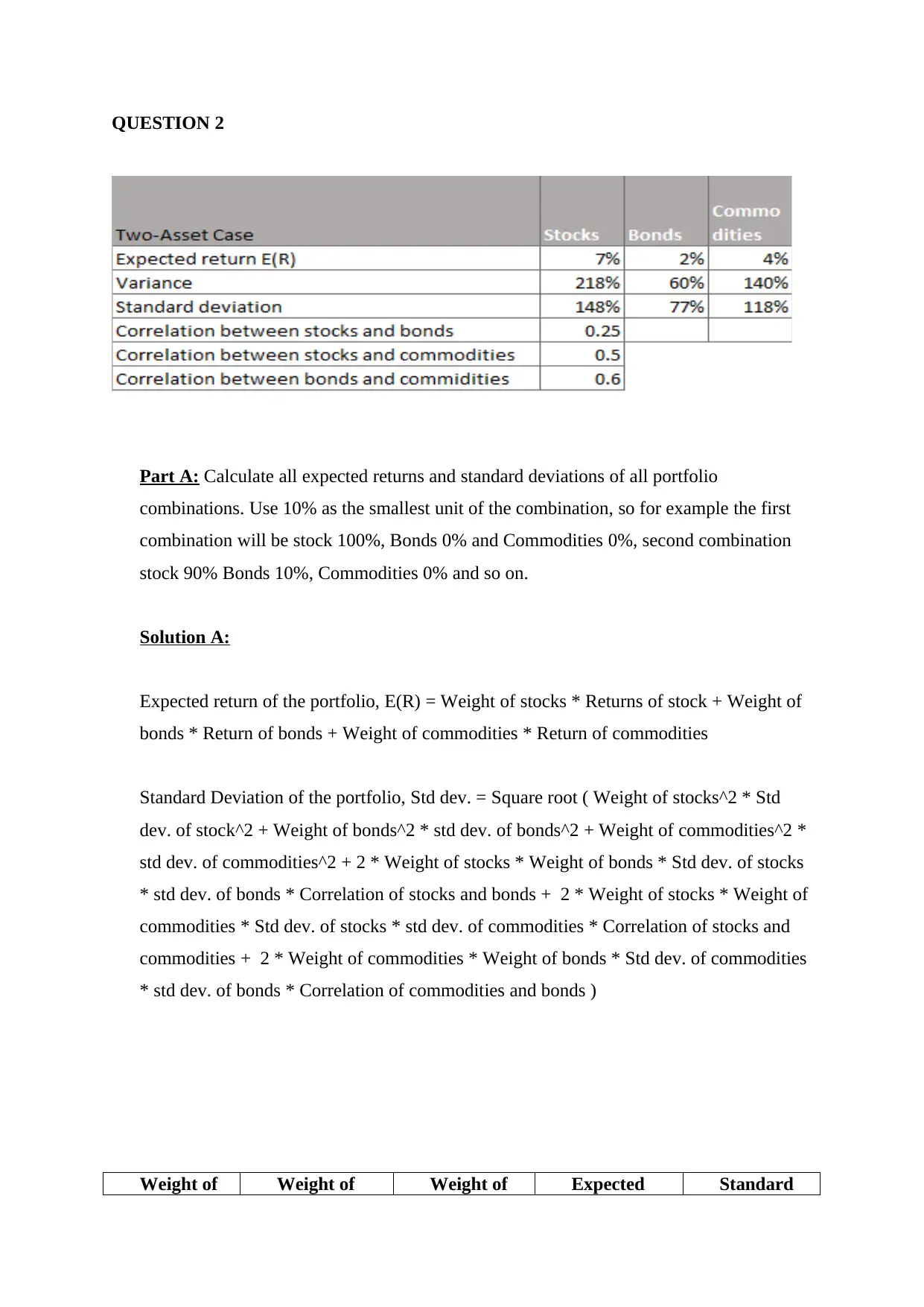
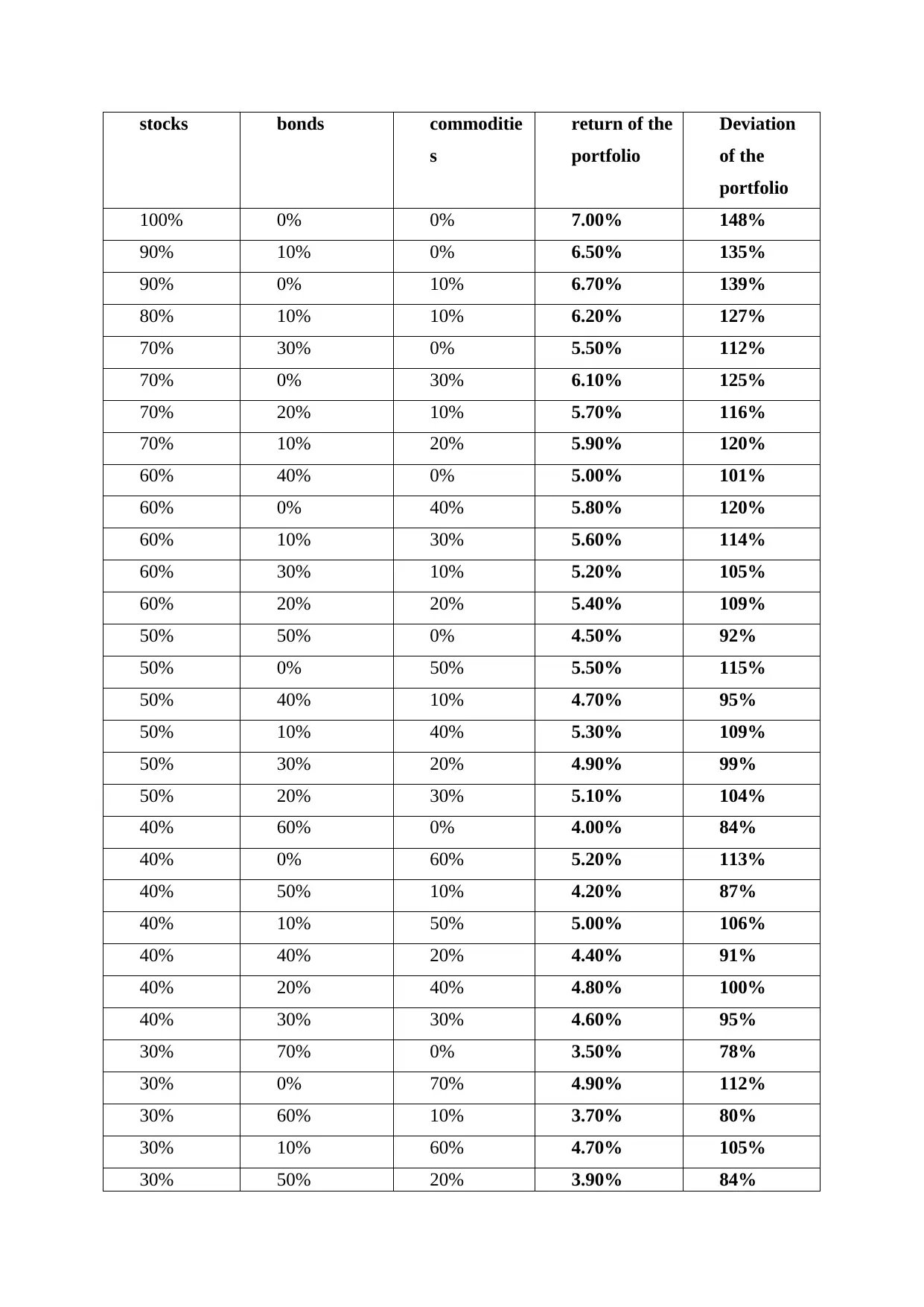
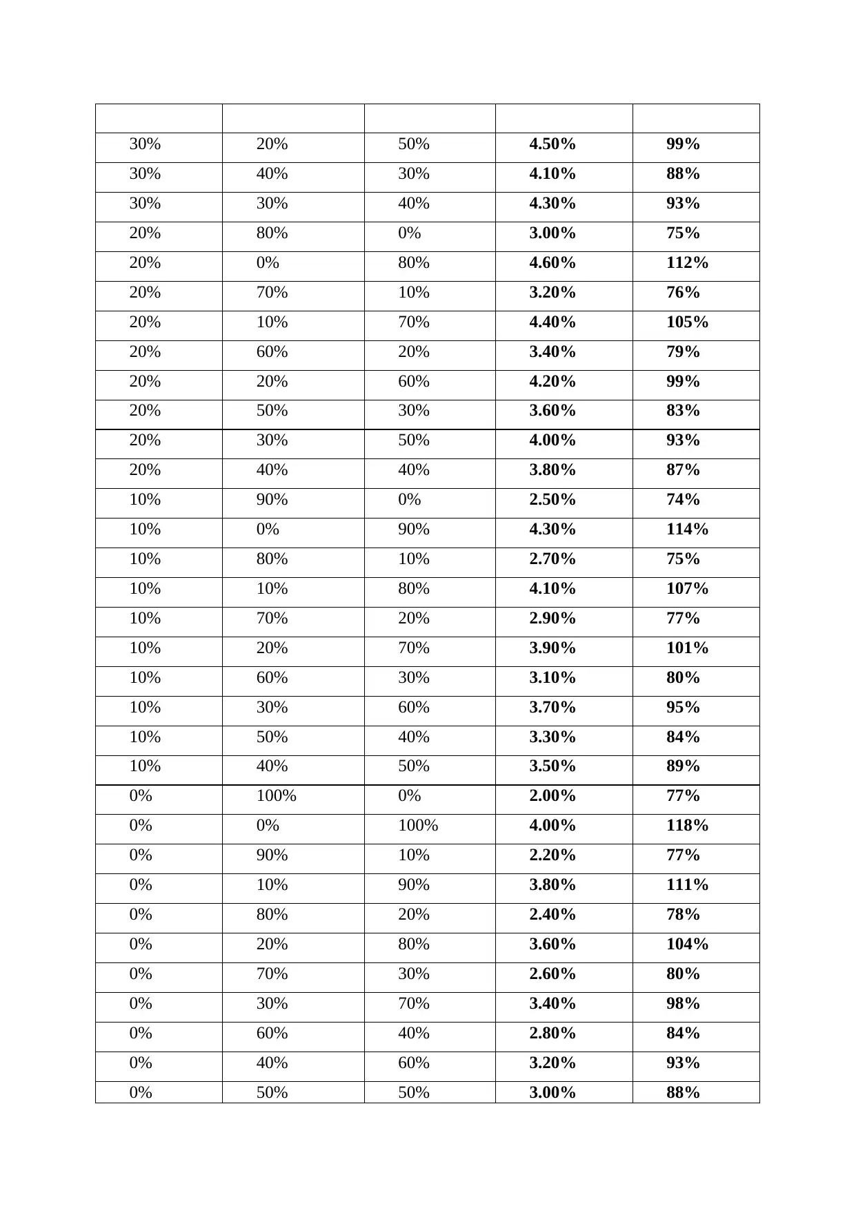
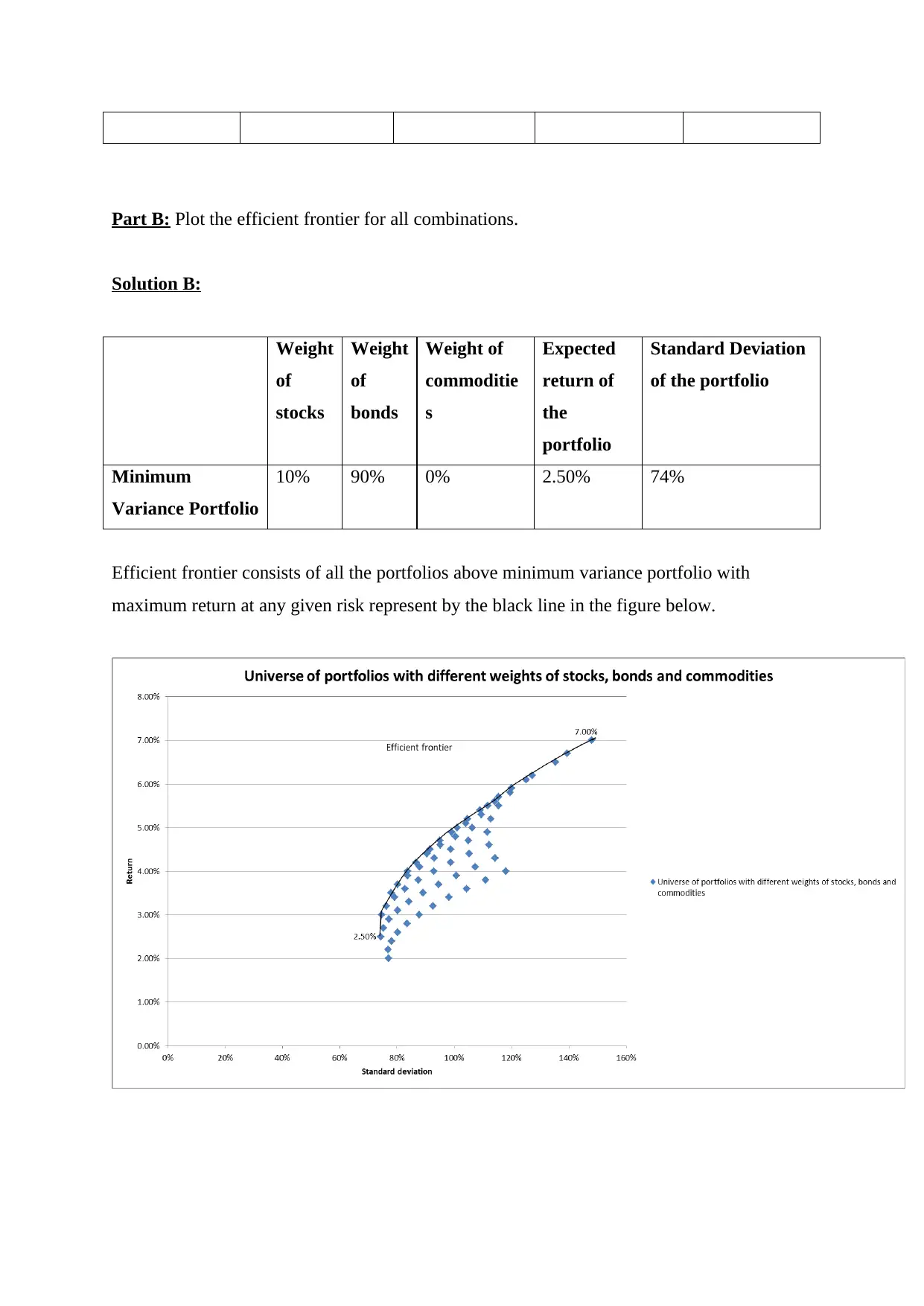
This project analyzes financial data, focusing on regression analysis and portfolio optimization. Question 1 involves predicting actual account balances based on computer-generated balances and calculating a 95% confidence interval for a specific account. Question 2 requires the calculation of expected returns and standard deviations for various portfolio combinations of stocks, bonds, and commodities. The analysis includes creating an efficient frontier to identify optimal portfolio allocations. The project utilizes regression equations and statistical methods to evaluate and optimize investment strategies, providing a comprehensive understanding of financial modeling and portfolio management.

(Details are shown in the excel file.)
QUESTION 1
Part A: If the computer-generated account balance was 120, what would you expect to be
the actual account balance as verified by the accountant?
Solution A:
Y: Actual account balance as verified by the accountant
X: Computer-generated account balance
Regression Equation, Y = 8.5513 + 1.0260 X
Given, X = 120
So, Y = 8.5513 + 1.0260 * 120 = 131.6713
Part B: The computer-generated balance for Oliver Buxton is listed as 100 in the
computer-generated account record. Calculate a 95% interval estimate for Mr. Buxton’s
actual account balance.
Solution B:
Y: Actual account balance as verified by the accountant
X: Computer-generated account balance
Regression Equation, Y = 8.5513 + 1.0260 X
Given, X = 100
So, Y = 8.5513 + 1.0260 * 100 = 111.1513
t-stat (at degree of freedom = number of observations-2 = 9) = 2.262157163

Standard error of regression = 13.73258073
95% confidence level of Actual account balance, Y = Predicted value of Y - ((t-stat at
given confidence level * standard error of regression or predicted value of Y)/ square root
(Number of observations)) to Predicted value of Y + ((t-stat at given confidence level *
standard error of regression or predicted value of Y)/ square root (Number of
observations))
95% confidence level of Actual account balance, Y = 111.1513 - ((2.262157163 *
13.73258073)/Square Root of (11)) to 111.1513 + ((2.262157163 * 13.73258073)/Square
Root of (11)) = 101.7847729 to 120.5178271

QUESTION 2
Part A: Calculate all expected returns and standard deviations of all portfolio
combinations. Use 10% as the smallest unit of the combination, so for example the first
combination will be stock 100%, Bonds 0% and Commodities 0%, second combination
stock 90% Bonds 10%, Commodities 0% and so on.
Solution A:
Expected return of the portfolio, E(R) = Weight of stocks * Returns of stock + Weight of
bonds * Return of bonds + Weight of commodities * Return of commodities
Standard Deviation of the portfolio, Std dev. = Square root ( Weight of stocks^2 * Std
dev. of stock^2 + Weight of bonds^2 * std dev. of bonds^2 + Weight of commodities^2 *
std dev. of commodities^2 + 2 * Weight of stocks * Weight of bonds * Std dev. of stocks
* std dev. of bonds * Correlation of stocks and bonds + 2 * Weight of stocks * Weight of
commodities * Std dev. of stocks * std dev. of commodities * Correlation of stocks and
commodities + 2 * Weight of commodities * Weight of bonds * Std dev. of commodities
* std dev. of bonds * Correlation of commodities and bonds )
Weight of Weight of Weight of Expected Standard

stocks bonds commoditie
s
return of the
portfolio
Deviation
of the
portfolio
100% 0% 0% 7.00% 148%
90% 10% 0% 6.50% 135%
90% 0% 10% 6.70% 139%
80% 10% 10% 6.20% 127%
70% 30% 0% 5.50% 112%
70% 0% 30% 6.10% 125%
70% 20% 10% 5.70% 116%
70% 10% 20% 5.90% 120%
60% 40% 0% 5.00% 101%
60% 0% 40% 5.80% 120%
60% 10% 30% 5.60% 114%
60% 30% 10% 5.20% 105%
60% 20% 20% 5.40% 109%
50% 50% 0% 4.50% 92%
50% 0% 50% 5.50% 115%
50% 40% 10% 4.70% 95%
50% 10% 40% 5.30% 109%
50% 30% 20% 4.90% 99%
50% 20% 30% 5.10% 104%
40% 60% 0% 4.00% 84%
40% 0% 60% 5.20% 113%
40% 50% 10% 4.20% 87%
40% 10% 50% 5.00% 106%
40% 40% 20% 4.40% 91%
40% 20% 40% 4.80% 100%
40% 30% 30% 4.60% 95%
30% 70% 0% 3.50% 78%
30% 0% 70% 4.90% 112%
30% 60% 10% 3.70% 80%
30% 10% 60% 4.70% 105%
30% 50% 20% 3.90% 84%

30% 20% 50% 4.50% 99%
30% 40% 30% 4.10% 88%
30% 30% 40% 4.30% 93%
20% 80% 0% 3.00% 75%
20% 0% 80% 4.60% 112%
20% 70% 10% 3.20% 76%
20% 10% 70% 4.40% 105%
20% 60% 20% 3.40% 79%
20% 20% 60% 4.20% 99%
20% 50% 30% 3.60% 83%
20% 30% 50% 4.00% 93%
20% 40% 40% 3.80% 87%
10% 90% 0% 2.50% 74%
10% 0% 90% 4.30% 114%
10% 80% 10% 2.70% 75%
10% 10% 80% 4.10% 107%
10% 70% 20% 2.90% 77%
10% 20% 70% 3.90% 101%
10% 60% 30% 3.10% 80%
10% 30% 60% 3.70% 95%
10% 50% 40% 3.30% 84%
10% 40% 50% 3.50% 89%
0% 100% 0% 2.00% 77%
0% 0% 100% 4.00% 118%
0% 90% 10% 2.20% 77%
0% 10% 90% 3.80% 111%
0% 80% 20% 2.40% 78%
0% 20% 80% 3.60% 104%
0% 70% 30% 2.60% 80%
0% 30% 70% 3.40% 98%
0% 60% 40% 2.80% 84%
0% 40% 60% 3.20% 93%
0% 50% 50% 3.00% 88%

Part B: Plot the efficient frontier for all combinations.
Solution B:
Weight
of
stocks
Weight
of
bonds
Weight of
commoditie
s
Expected
return of
the
portfolio
Standard Deviation
of the portfolio
Minimum
Variance Portfolio
10% 90% 0% 2.50% 74%
Efficient frontier consists of all the portfolios above minimum variance portfolio with
maximum return at any given risk represent by the black line in the figure below.