University Financial Statistics Report: Sales Data Analysis FIN10002

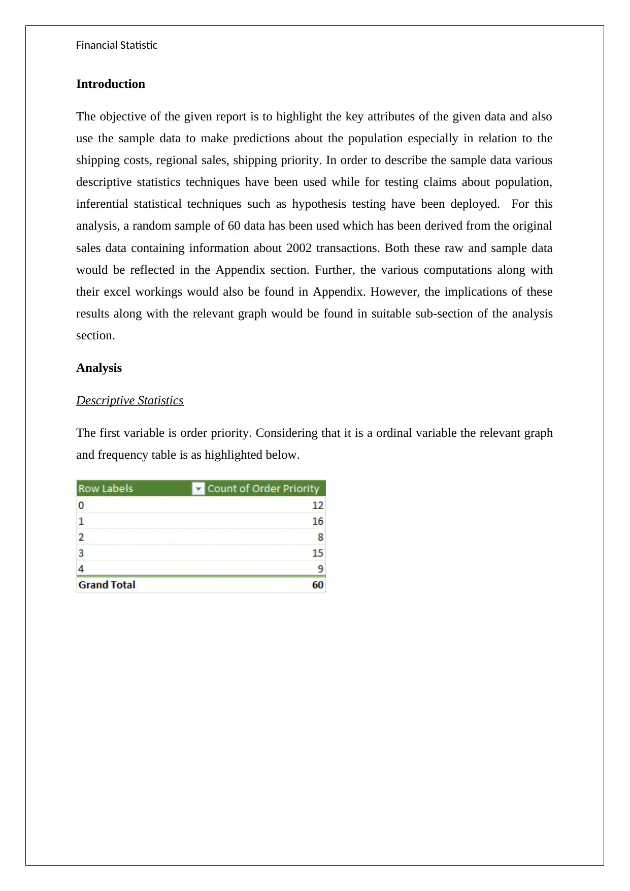
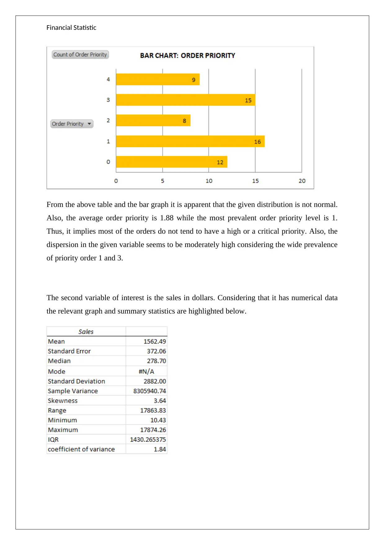
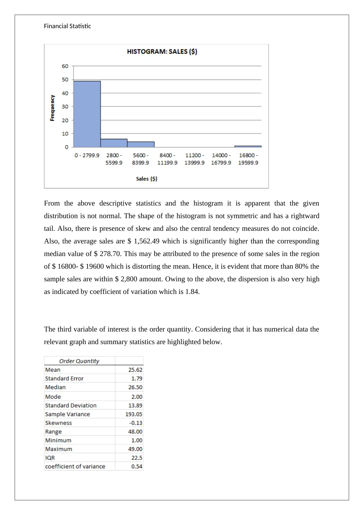
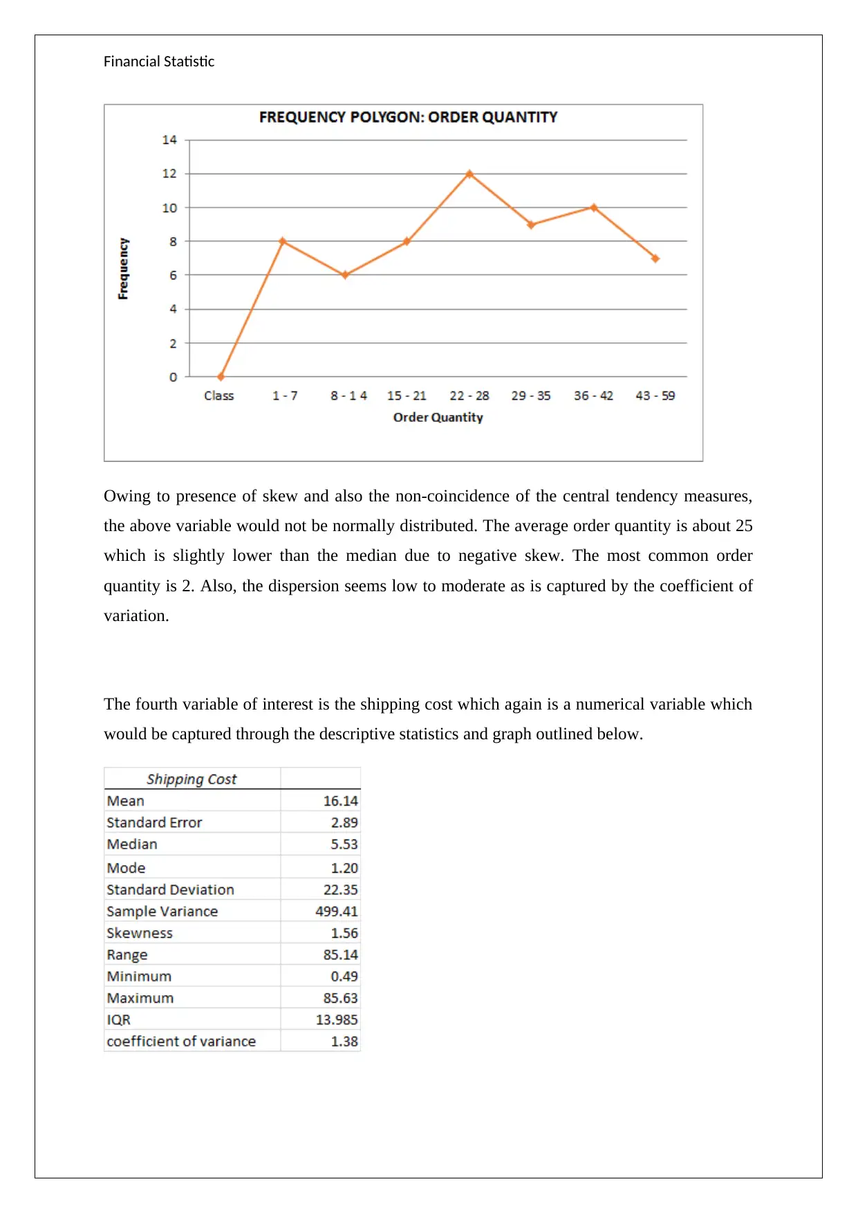
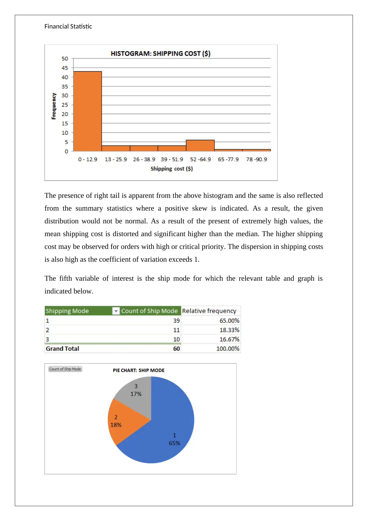
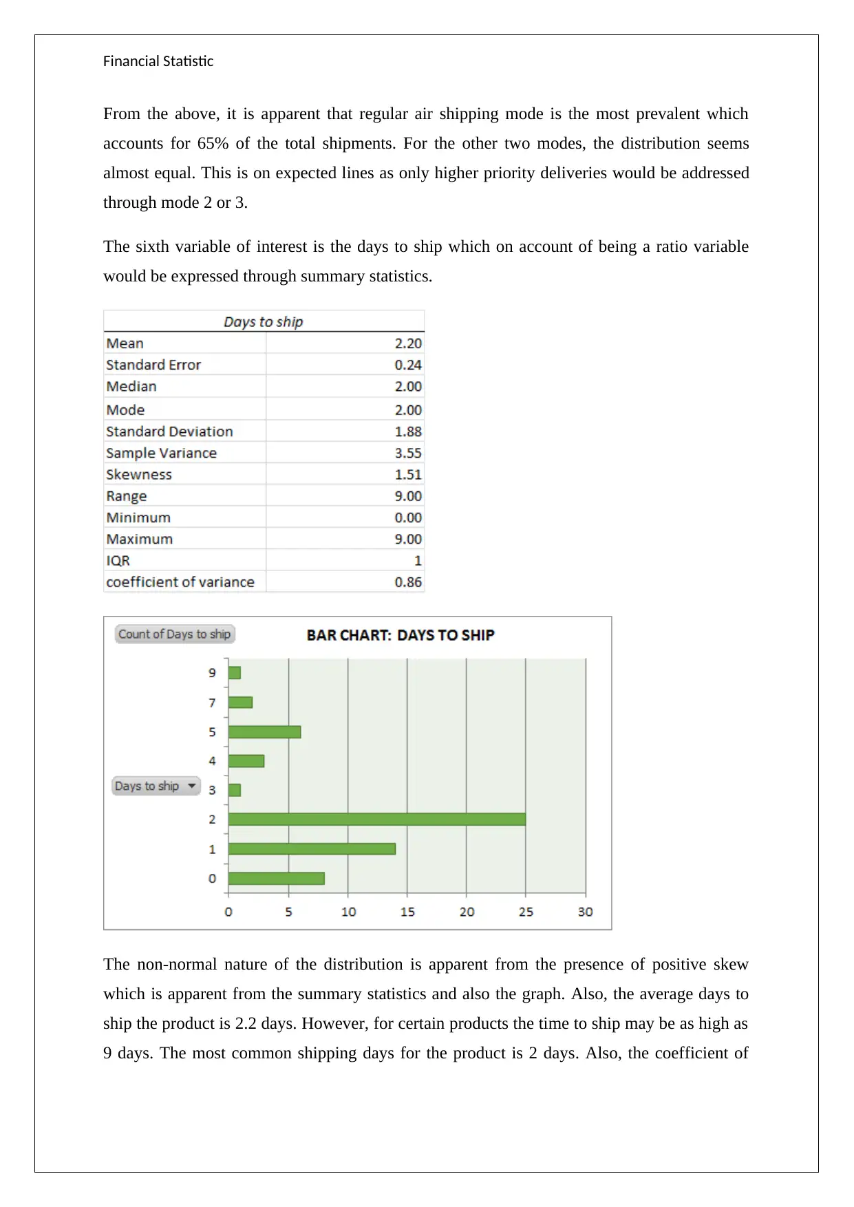
This report presents a statistical analysis of sales data, employing both descriptive and inferential statistical techniques. The analysis includes summarizing variables using computational and graphical tools, such as order priority, sales in dollars, order quantity, shipping cost, ship mode, days to ship, region of sales, and customer segment. Inferential statistics is used to test claims about sales population data, calculate confidence intervals for the mean, and perform hypothesis tests. The report also explores the relationship between order quantity and sales using linear regression. The findings indicate that the hypothesis tests did not support the claims made, although confidence intervals appeared accurate. The regression analysis did not yield a statistically significant relationship between order quantity and sales. The report acknowledges that the historical nature of the data might limit the relevance of the results to current market trends. The appendix includes the raw and sample data, along with the Excel workings.

FINANCIAL STATISTICS
FIN10002
STUDENT ID:
[Pick the date]

Financial Statistic
Executive Summary
The given report aims to carry a statistical analysis of the sample data pertaining to the sale of
supplies. In this process, various descriptive and inferential statistical techniques have been
deployed. The various variables in the sample data have been summarised using appropriate
computational and graphical tools available under the aegis of descriptive statistics. Further,
using the inferential statistics technique various claims have been tested with regards to the
sales population data and also appropriate intervals for mean have been determined. The
hypothesis tests conducted do not suggest any support for the claims made. However, the
confidence interval determined seems accurate as has been verified from the population data.
Also, linear regression has been done to highlight the nature and extent of relationship
between the order quantity and sales but this did not yield any statistically significant
relationship. These results though valid may have limited relevance owing to the data being
historically quite old and hence the current patterns and observations may deviate
significantly from the sample or population data taken into consideration.

Financial Statistic
Introduction
The objective of the given report is to highlight the key attributes of the given data and also
use the sample data to make predictions about the population especially in relation to the
shipping costs, regional sales, shipping priority. In order to describe the sample data various
descriptive statistics techniques have been used while for testing claims about population,
inferential statistical techniques such as hypothesis testing have been deployed. For this
analysis, a random sample of 60 data has been used which has been derived from the original
sales data containing information about 2002 transactions. Both these raw and sample data
would be reflected in the Appendix section. Further, the various computations along with
their excel workings would also be found in Appendix. However, the implications of these
results along with the relevant graph would be found in suitable sub-section of the analysis
section.
Analysis
Descriptive Statistics
The first variable is order priority. Considering that it is a ordinal variable the relevant graph
and frequency table is as highlighted below.

Financial Statistic
From the above table and the bar graph it is apparent that the given distribution is not normal.
Also, the average order priority is 1.88 while the most prevalent order priority level is 1.
Thus, it implies most of the orders do not tend to have a high or a critical priority. Also, the
dispersion in the given variable seems to be moderately high considering the wide prevalence
of priority order 1 and 3.
The second variable of interest is the sales in dollars. Considering that it has numerical data
the relevant graph and summary statistics are highlighted below.

Financial Statistic
From the above descriptive statistics and the histogram it is apparent that the given
distribution is not normal. The shape of the histogram is not symmetric and has a rightward
tail. Also, there is presence of skew and also the central tendency measures do not coincide.
Also, the average sales are $ 1,562.49 which is significantly higher than the corresponding
median value of $ 278.70. This may be attributed to the presence of some sales in the region
of $ 16800- $ 19600 which is distorting the mean. Hence, it is evident that more than 80% the
sample sales are within $ 2,800 amount. Owing to the above, the dispersion is also very high
as indicated by coefficient of variation which is 1.84.
The third variable of interest is the order quantity. Considering that it has numerical data the
relevant graph and summary statistics are highlighted below.

Financial Statistic
Owing to presence of skew and also the non-coincidence of the central tendency measures,
the above variable would not be normally distributed. The average order quantity is about 25
which is slightly lower than the median due to negative skew. The most common order
quantity is 2. Also, the dispersion seems low to moderate as is captured by the coefficient of
variation.
The fourth variable of interest is the shipping cost which again is a numerical variable which
would be captured through the descriptive statistics and graph outlined below.

Financial Statistic
The presence of right tail is apparent from the above histogram and the same is also reflected
from the summary statistics where a positive skew is indicated. As a result, the given
distribution would not be normal. As a result of the present of extremely high values, the
mean shipping cost is distorted and significant higher than the median. The higher shipping
cost may be observed for orders with high or critical priority. The dispersion in shipping costs
is also high as the coefficient of variation exceeds 1.
The fifth variable of interest is the ship mode for which the relevant table and graph is
indicated below.

Financial Statistic
From the above, it is apparent that regular air shipping mode is the most prevalent which
accounts for 65% of the total shipments. For the other two modes, the distribution seems
almost equal. This is on expected lines as only higher priority deliveries would be addressed
through mode 2 or 3.
The sixth variable of interest is the days to ship which on account of being a ratio variable
would be expressed through summary statistics.
The non-normal nature of the distribution is apparent from the presence of positive skew
which is apparent from the summary statistics and also the graph. Also, the average days to
ship the product is 2.2 days. However, for certain products the time to ship may be as high as
9 days. The most common shipping days for the product is 2 days. Also, the coefficient of

Financial Statistic
variation seems to be moderately high but it is less than 1 indicating moderate to high
dispersion in the given data.
The seventh variable of interest is the region of sales for which the requisite graph along with
the frequency table is as indicated below.
It is apparent from the above graph and table that about 63% of the products are delivered to
a Eastern state and only 37% of these are delivered to a Western state.
The last variable of interest is the customer segment which would be captured through the
frequency table and the representative graph as highlighted below.

Financial Statistic
It is apparent from the above that about 50% of the customers comprise of the corporate
segment while the representation of the remaining segments is almost equal with no
significant difference visible in the given sample.
Confidence Interval
We are 95% confident that the average sales amount from the orders obtained from home
office customers only would lie between $ 363.48 and $ 3,472.73. The corresponding
population mean comes out as $ 1,585.08. This clearly highlights that the confidence interval
seems accurate since the population mean does tend to lie within the interval predicted and
that too about the middle thus indicating similarity between population and sample mean.
We are 95% confidence that the average shipping cost per order would lie between $10.37
and $ 21.91. The corresponding population mean comes out as $ 12.45. This clearly
highlights that the confidence interval seems accurate since the population mean does tend to
lie within the interval predicted.
Hypothesis Testing
From the given sample data, hypothesis testing has been used so as to derive conclusions
about the population using hypothesis testing where the null hypothesis is tested and in case
of the rejection of the same the alternative hypothesis is accepted. Based on the relevant
computations highlighted in the appendix, it may be concluded with 95% confidence that

Financial Statistic
there is no statistically significant difference between the average shipping costs for critical
priority orders and low priority orders. Also, the relevant computations highlight with 95%
confidence that there is statistically significant difference between the average sales order ($)
from the Eastern and Western states. Thus, both the claims tested have been not supported by
the given sample data.
Correlation and Regression
The requisite scatterplot is as outlined below.
It is apparent from the positive sloping best fit line that there is a positive relationship
between order quantity and sales. However, the relationship is quite weak which is apparent
from the high amount of deviation from the line of best fit and also the corresponding
coefficient of determination.
The regression equation has been highlighted in the scatterplot and has also been derived
from the linear regression in excel. The coefficient of determination or R2 highlights that only
3.06% of the changes in sales are accounted for by corresponding changes in the order
quantity. Also, the correlation coefficient for the given variables is low at 0.17 which is
representative of only weak positive correlation between the given variables. The intercept of
633.34 highlights the sales when the order quantity is zero and is not practical. Further, the
slope highlights that with a unit increase in the order quantity, the sales would increase by $
36.27. Besides, the hypothesis testing for regression model significance suggests that the
slope is not significant and hence it can be assumed as zero. This implies that the given

Financial Statistic
regression model is not significance which implies that the relationship between order
quantity and sales is not statistically significant.
Conclusion
Based on the given discussion, it is apparent that the confidence intervals which have been
determined based on the sample data are quite accurate which is apparent from the respective
comparison with the actual population mean. Further, there is no significant difference
observed between the average sales generated from eastern and western states. Also, the
shipping costs related to the different priority orders also do not show any significant
difference. Besides, the regression model has also not been found to be significant
considering the hypothesis testing and the values of R and R2. Even though the sample size
was small but it was representative of the overall population. However, the data might not be
relevant any longer considering that it is historical data and the trends may have changed
since then. Hence, it is advisable that the recent or latest data in this regards should have been
taken for more relevant results.
Appendix
Random Sample