Financial Statement Analysis and Investment Appraisal Report
VerifiedAdded on 2021/02/21
|17
|5128
|72
Report
AI Summary
This report provides an in-depth analysis of financial statements, including income statements and balance sheets, for Yarnshaw Limited. It covers the calculation of key financial metrics and the preparation of these statements. The report further delves into management accounting concepts, models, and techniques, using Reckturk Plc as a case study to illustrate break-even analysis, margin of safety, and profit calculations. It also explores various investment appraisal techniques, their merits, demerits, and the benefits and limitations of budgeting. The report aims to provide a comprehensive understanding of financial accounting, management accounting, and investment decision-making processes. It includes detailed working notes and calculations to support the financial analyses presented.

INTRODUCTION TO
ACCOUNTING AND
FINANCE
ACCOUNTING AND
FINANCE
Paraphrase This Document
Need a fresh take? Get an instant paraphrase of this document with our AI Paraphraser

TABLE OF CONTENTS
INTRODUCTION...........................................................................................................................1
PART A -Yarnshaw Limited...........................................................................................................1
PART B – Reckturk Plc...................................................................................................................5
PART C............................................................................................................................................9
A. Calculation of investment appraisal techniques......................................................................9
B. Merits and demerits of different investment appraisal techniques........................................11
C. Explain the benefits and limitation of Budget.......................................................................12
CONCLUSION..............................................................................................................................13
REFERENCES..............................................................................................................................14
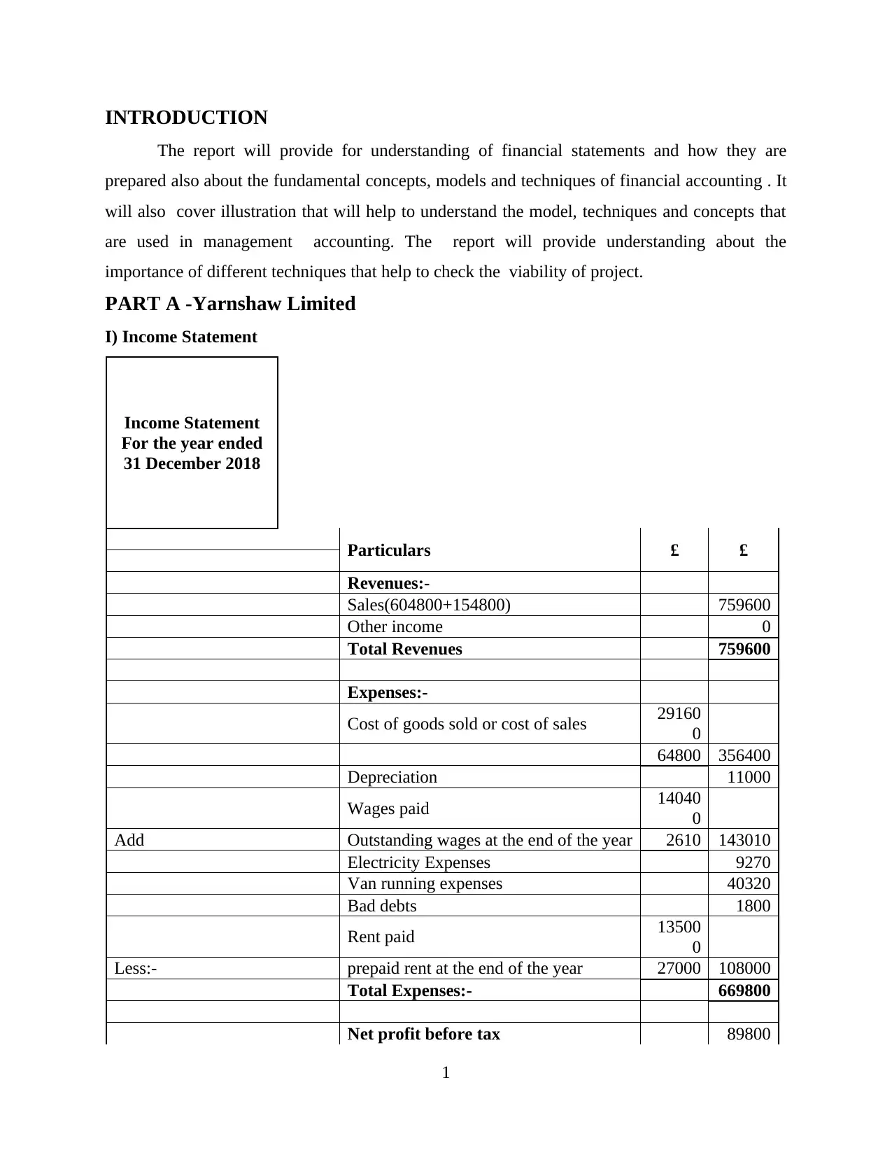
INTRODUCTION
The report will provide for understanding of financial statements and how they are
prepared also about the fundamental concepts, models and techniques of financial accounting . It
will also cover illustration that will help to understand the model, techniques and concepts that
are used in management accounting. The report will provide understanding about the
importance of different techniques that help to check the viability of project.
PART A -Yarnshaw Limited
I) Income Statement
Income Statement
For the year ended
31 December 2018
Particulars £ £
Revenues:-
Sales(604800+154800) 759600
Other income 0
Total Revenues 759600
Expenses:-
Cost of goods sold or cost of sales 29160
0
64800 356400
Depreciation 11000
Wages paid 14040
0
Add Outstanding wages at the end of the year 2610 143010
Electricity Expenses 9270
Van running expenses 40320
Bad debts 1800
Rent paid 13500
0
Less:- prepaid rent at the end of the year 27000 108000
Total Expenses:- 669800
Net profit before tax 89800
1
⊘ This is a preview!⊘
Do you want full access?
Subscribe today to unlock all pages.
Trusted by 1+ million students worldwide
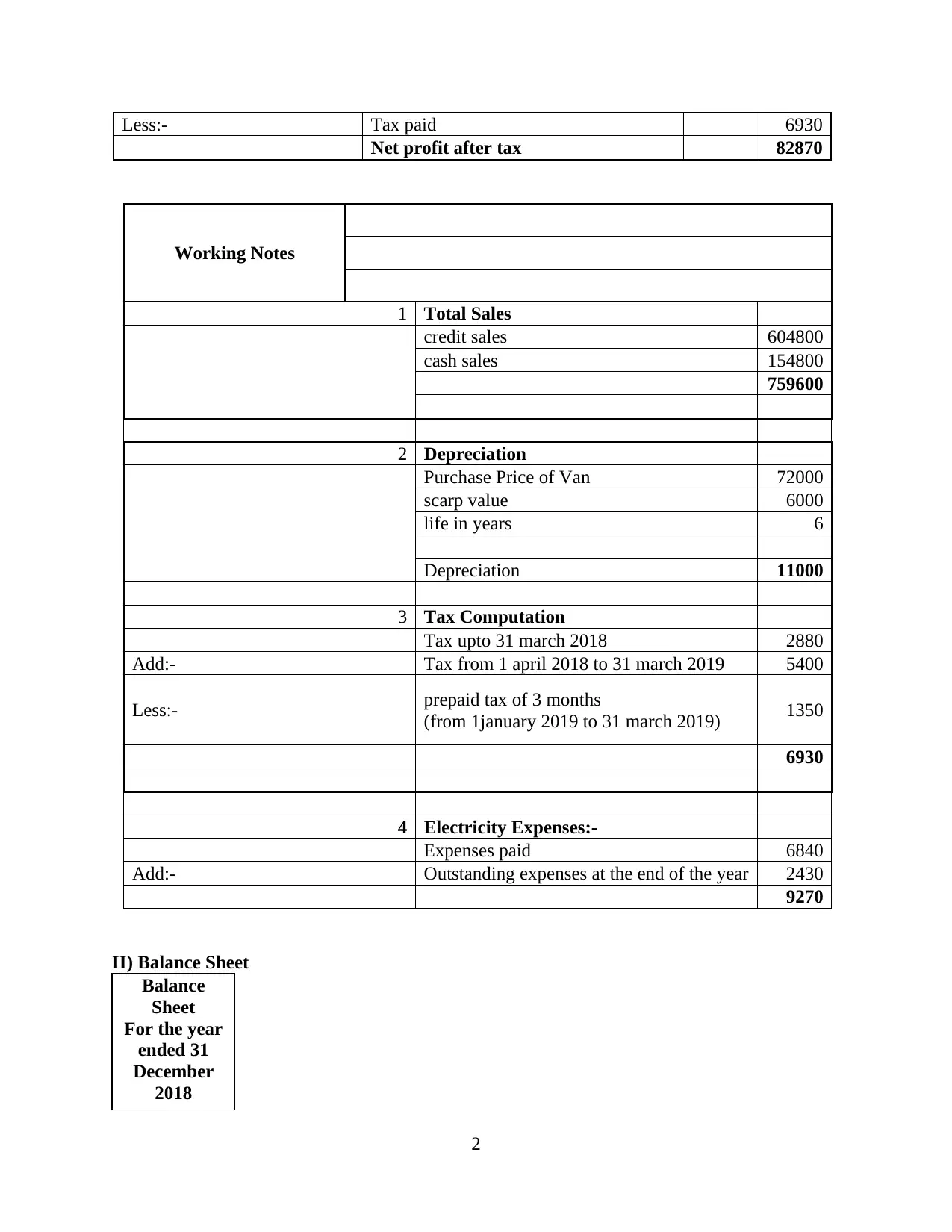
Less:- Tax paid 6930
Net profit after tax 82870
Working Notes
1 Total Sales
credit sales 604800
cash sales 154800
759600
2 Depreciation
Purchase Price of Van 72000
scarp value 6000
life in years 6
Depreciation 11000
3 Tax Computation
Tax upto 31 march 2018 2880
Add:- Tax from 1 april 2018 to 31 march 2019 5400
Less:- prepaid tax of 3 months
(from 1january 2019 to 31 march 2019) 1350
6930
4 Electricity Expenses:-
Expenses paid 6840
Add:- Outstanding expenses at the end of the year 2430
9270
II) Balance Sheet
Balance
Sheet
For the year
ended 31
December
2018
2
Paraphrase This Document
Need a fresh take? Get an instant paraphrase of this document with our AI Paraphraser
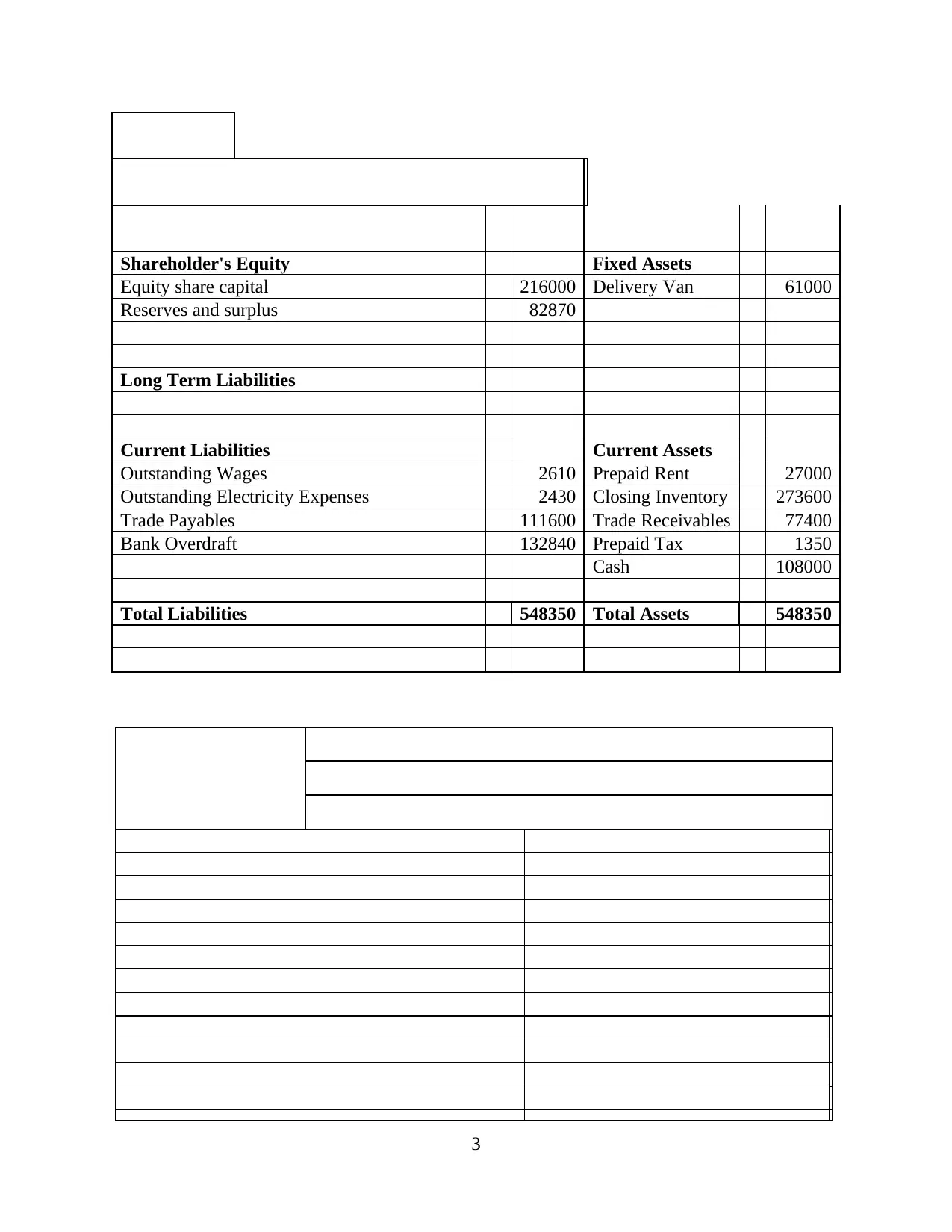
Shareholder's Equity Fixed Assets
Equity share capital 216000 Delivery Van 61000
Reserves and surplus 82870
Long Term Liabilities
Current Liabilities Current Assets
Outstanding Wages 2610 Prepaid Rent 27000
Outstanding Electricity Expenses 2430 Closing Inventory 273600
Trade Payables 111600 Trade Receivables 77400
Bank Overdraft 132840 Prepaid Tax 1350
Cash 108000
Total Liabilities 548350 Total Assets 548350
3
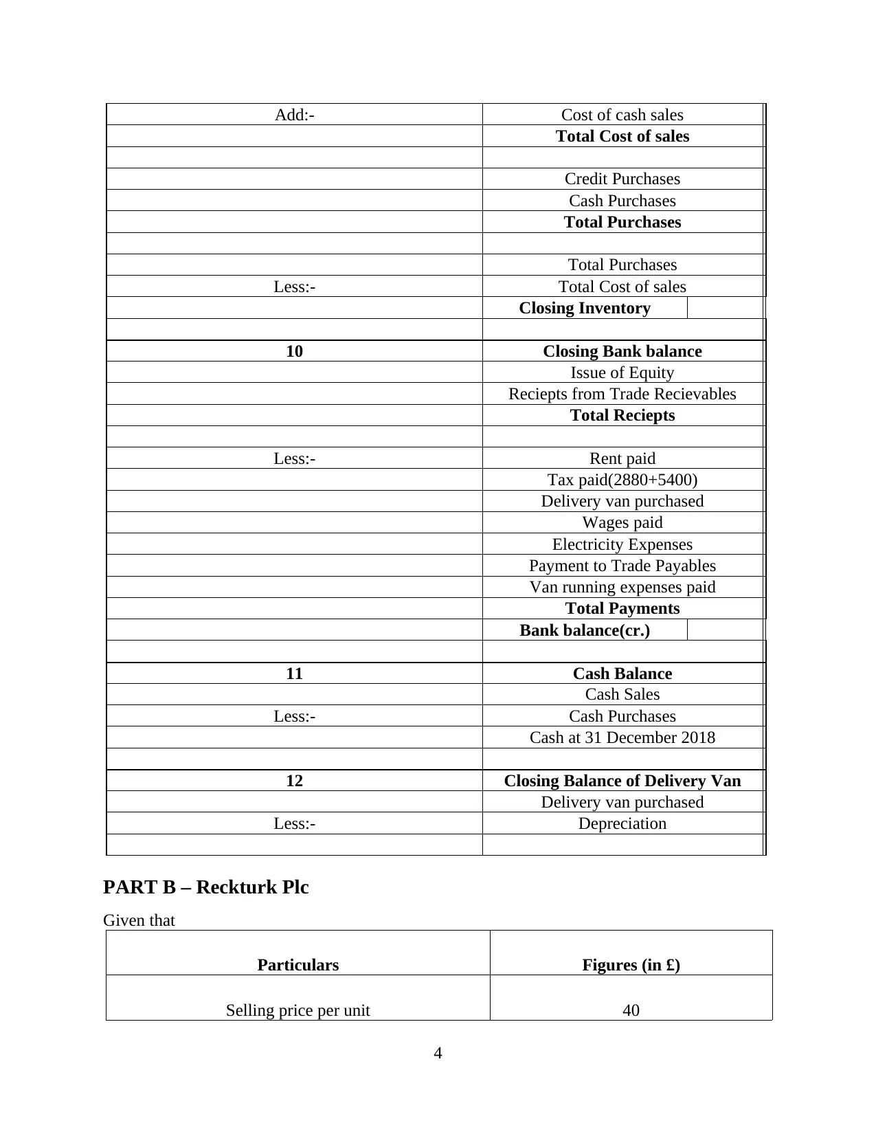
Add:- Cost of cash sales
Total Cost of sales
Credit Purchases
Cash Purchases
Total Purchases
Total Purchases
Less:- Total Cost of sales
Closing Inventory
10 Closing Bank balance
Issue of Equity
Reciepts from Trade Recievables
Total Reciepts
Less:- Rent paid
Tax paid(2880+5400)
Delivery van purchased
Wages paid
Electricity Expenses
Payment to Trade Payables
Van running expenses paid
Total Payments
Bank balance(cr.)
11 Cash Balance
Cash Sales
Less:- Cash Purchases
Cash at 31 December 2018
12 Closing Balance of Delivery Van
Delivery van purchased
Less:- Depreciation
PART B – Reckturk Plc
Given that
Particulars Figures (in £)
Selling price per unit 40
4
⊘ This is a preview!⊘
Do you want full access?
Subscribe today to unlock all pages.
Trusted by 1+ million students worldwide
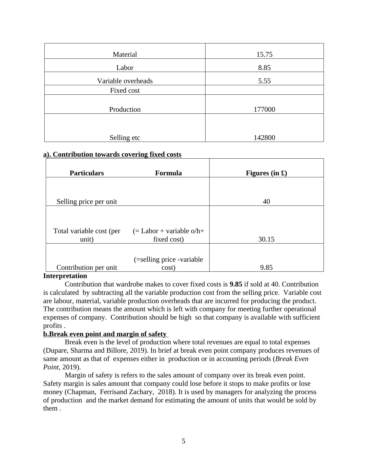
Material 15.75
Labor 8.85
Variable overheads 5.55
Fixed cost
Production 177000
Selling etc 142800
a). Contribution towards covering fixed costs
Particulars Formula Figures (in £)
Selling price per unit 40
Total variable cost (per
unit)
(= Labor + variable o/h+
fixed cost) 30.15
Contribution per unit
(=selling price -variable
cost) 9.85
Interpretation
Contribution that wardrobe makes to cover fixed costs is 9.85 if sold at 40. Contribution
is calculated by subtracting all the variable production cost from the selling price. Variable cost
are labour, material, variable production overheads that are incurred for producing the product.
The contribution means the amount which is left with company for meeting further operational
expenses of company. Contribution should be high so that company is available with sufficient
profits .
b.Break even point and margin of safety
Break even is the level of production where total revenues are equal to total expenses
(Dupare, Sharma and Billore, 2019). In brief at break even point company produces revenues of
same amount as that of expenses either in production or in accounting periods (Break Even
Point, 2019).
Margin of safety is refers to the sales amount of company over its break even point.
Safety margin is sales amount that company could lose before it stops to make profits or lose
money (Chapman, Ferrisand Zachary, 2018). It is used by managers for analyzing the process
of production and the market demand for estimating the amount of units that would be sold by
them .
5
Paraphrase This Document
Need a fresh take? Get an instant paraphrase of this document with our AI Paraphraser
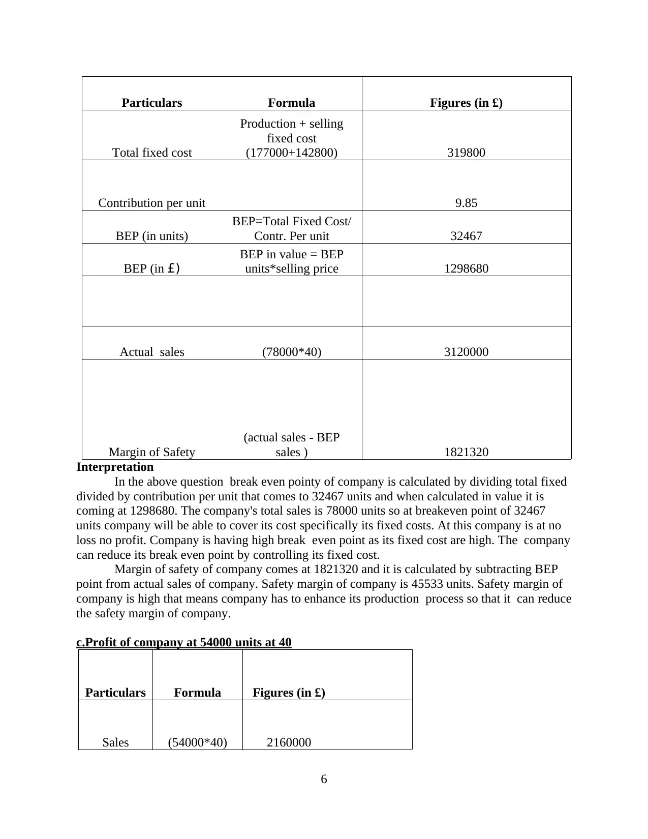
Particulars Formula Figures (in £)
Total fixed cost
Production + selling
fixed cost
(177000+142800) 319800
Contribution per unit 9.85
BEP (in units)
BEP=Total Fixed Cost/
Contr. Per unit 32467
BEP (in £)
BEP in value = BEP
units*selling price 1298680
Actual sales (78000*40) 3120000
Margin of Safety
(actual sales - BEP
sales ) 1821320
Interpretation
In the above question break even pointy of company is calculated by dividing total fixed
divided by contribution per unit that comes to 32467 units and when calculated in value it is
coming at 1298680. The company's total sales is 78000 units so at breakeven point of 32467
units company will be able to cover its cost specifically its fixed costs. At this company is at no
loss no profit. Company is having high break even point as its fixed cost are high. The company
can reduce its break even point by controlling its fixed cost.
Margin of safety of company comes at 1821320 and it is calculated by subtracting BEP
point from actual sales of company. Safety margin of company is 45533 units. Safety margin of
company is high that means company has to enhance its production process so that it can reduce
the safety margin of company.
c.Profit of company at 54000 units at 40
Particulars Formula Figures (in £)
Sales (54000*40) 2160000
6

Material (54000*15.75) 850500
Labor (54000*8.85) 477900
Variable
overheads (54000*5.55) 299700
Contributio
n 531900
Fixed cost
Production 177000
Selling etc 142800
Profit 212100
Interpretation
If the company is producing 54000 units of wardrobe it will be able to produce profits of
212100. The variable cost of the company will remain same for producing 54000 units as
variable remains constant and do not change with change in increase or decrease of production
units where fixed cost remains constant in total but changes per unit.
d).
7
⊘ This is a preview!⊘
Do you want full access?
Subscribe today to unlock all pages.
Trusted by 1+ million students worldwide
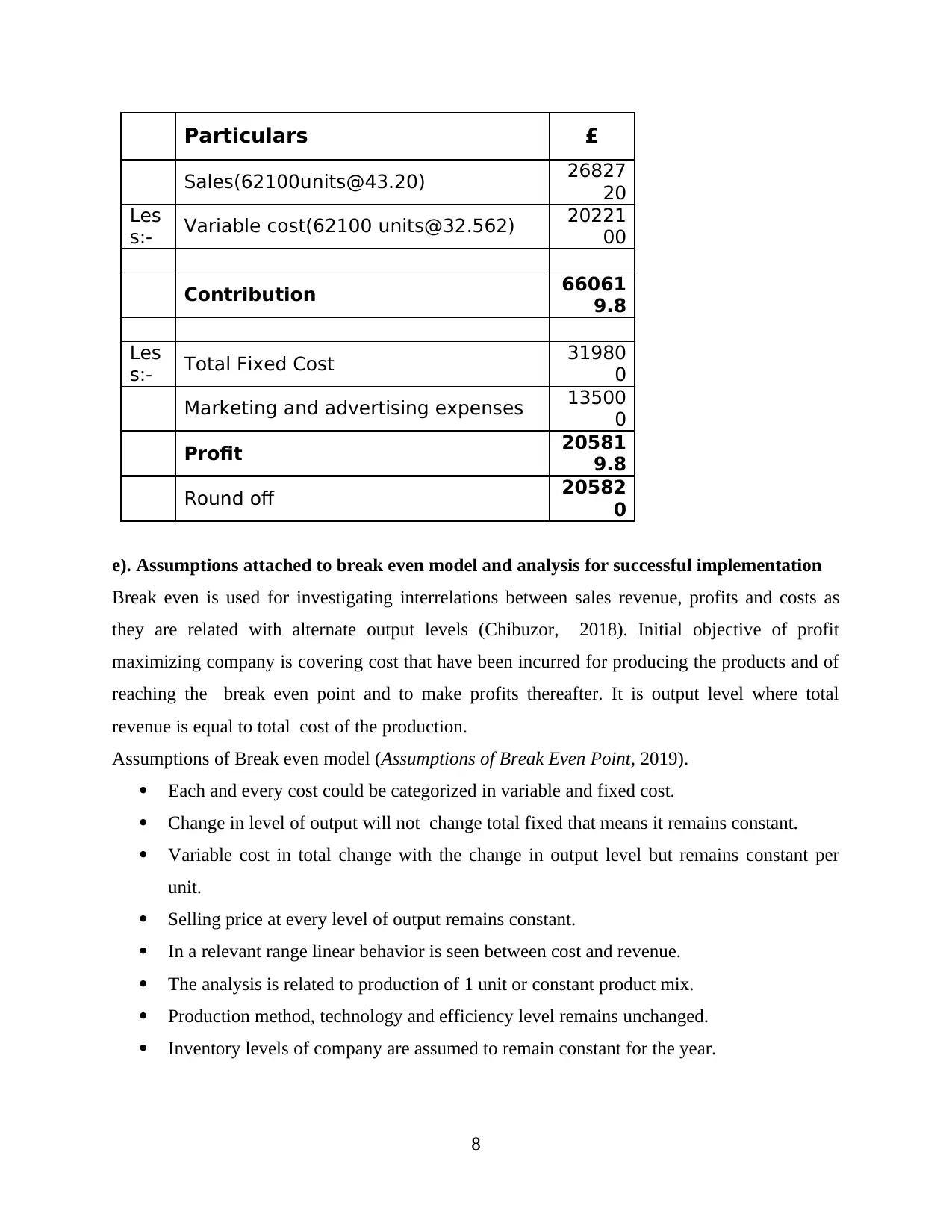
Particulars £
Sales(62100units@43.20) 26827
20
Les
s:- Variable cost(62100 units@32.562) 20221
00
Contribution 66061
9.8
Les
s:- Total Fixed Cost 31980
0
Marketing and advertising expenses 13500
0
Profit 20581
9.8
Round off 20582
0
e). Assumptions attached to break even model and analysis for successful implementation
Break even is used for investigating interrelations between sales revenue, profits and costs as
they are related with alternate output levels (Chibuzor, 2018). Initial objective of profit
maximizing company is covering cost that have been incurred for producing the products and of
reaching the break even point and to make profits thereafter. It is output level where total
revenue is equal to total cost of the production.
Assumptions of Break even model (Assumptions of Break Even Point, 2019).
Each and every cost could be categorized in variable and fixed cost.
Change in level of output will not change total fixed that means it remains constant.
Variable cost in total change with the change in output level but remains constant per
unit.
Selling price at every level of output remains constant.
In a relevant range linear behavior is seen between cost and revenue.
The analysis is related to production of 1 unit or constant product mix.
Production method, technology and efficiency level remains unchanged.
Inventory levels of company are assumed to remain constant for the year.
8
Paraphrase This Document
Need a fresh take? Get an instant paraphrase of this document with our AI Paraphraser
The model can be used by manufacturing companies for calculating per unit costs, break
even points and for analyzing whether company is able to produce required number of units for
covering its costs (Dillon and Casey, 2016). The model can be used different business that are
involved in production of goods where the method is not successful for service industry. In
service industry it is critical for company to come at break even point as it is difficult for those
company to bifurcate variable and fixed costs (Massol, Tchung-Ming and Banal-Estanol, 2018).
PART C
A. Calculation of investment appraisal techniques
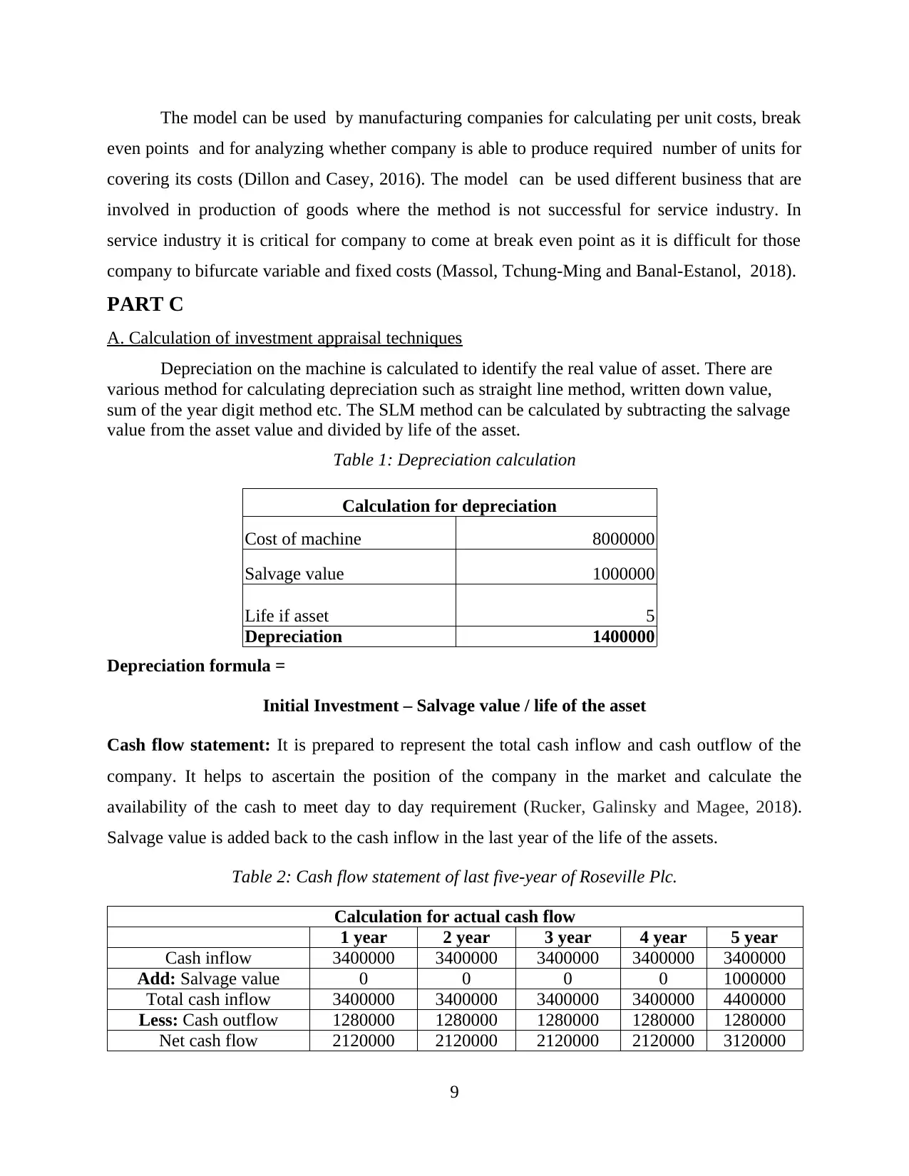
Depreciation on the machine is calculated to identify the real value of asset. There are
various method for calculating depreciation such as straight line method, written down value,
sum of the year digit method etc. The SLM method can be calculated by subtracting the salvage
value from the asset value and divided by life of the asset.
Table 1: Depreciation calculation
Calculation for depreciation
Cost of machine 8000000
Salvage value 1000000
Life if asset 5
Depreciation 1400000
Depreciation formula =
Initial Investment – Salvage value / life of the asset
Cash flow statement: It is prepared to represent the total cash inflow and cash outflow of the
company. It helps to ascertain the position of the company in the market and calculate the
availability of the cash to meet day to day requirement (Rucker, Galinsky and Magee, 2018).
Salvage value is added back to the cash inflow in the last year of the life of the assets.
Table 2: Cash flow statement of last five-year of Roseville Plc.
Calculation for actual cash flow
1 year 2 year 3 year 4 year 5 year
Cash inflow 3400000 3400000 3400000 3400000 3400000
Add: Salvage value 0 0 0 0 1000000
Total cash inflow 3400000 3400000 3400000 3400000 4400000
Less: Cash outflow 1280000 1280000 1280000 1280000 1280000
Net cash flow 2120000 2120000 2120000 2120000 3120000
9
even points and for analyzing whether company is able to produce required number of units for
covering its costs (Dillon and Casey, 2016). The model can be used different business that are
involved in production of goods where the method is not successful for service industry. In
service industry it is critical for company to come at break even point as it is difficult for those
company to bifurcate variable and fixed costs (Massol, Tchung-Ming and Banal-Estanol, 2018).
PART C
A. Calculation of investment appraisal techniques
Depreciation on the machine is calculated to identify the real value of asset. There are
various method for calculating depreciation such as straight line method, written down value,
sum of the year digit method etc. The SLM method can be calculated by subtracting the salvage
value from the asset value and divided by life of the asset.
Table 1: Depreciation calculation
Calculation for depreciation
Cost of machine 8000000
Salvage value 1000000
Life if asset 5
Depreciation 1400000
Depreciation formula =
Initial Investment – Salvage value / life of the asset
Cash flow statement: It is prepared to represent the total cash inflow and cash outflow of the
company. It helps to ascertain the position of the company in the market and calculate the
availability of the cash to meet day to day requirement (Rucker, Galinsky and Magee, 2018).
Salvage value is added back to the cash inflow in the last year of the life of the assets.
Table 2: Cash flow statement of last five-year of Roseville Plc.
Calculation for actual cash flow
1 year 2 year 3 year 4 year 5 year
Cash inflow 3400000 3400000 3400000 3400000 3400000
Add: Salvage value 0 0 0 0 1000000
Total cash inflow 3400000 3400000 3400000 3400000 4400000
Less: Cash outflow 1280000 1280000 1280000 1280000 1280000
Net cash flow 2120000 2120000 2120000 2120000 3120000
9
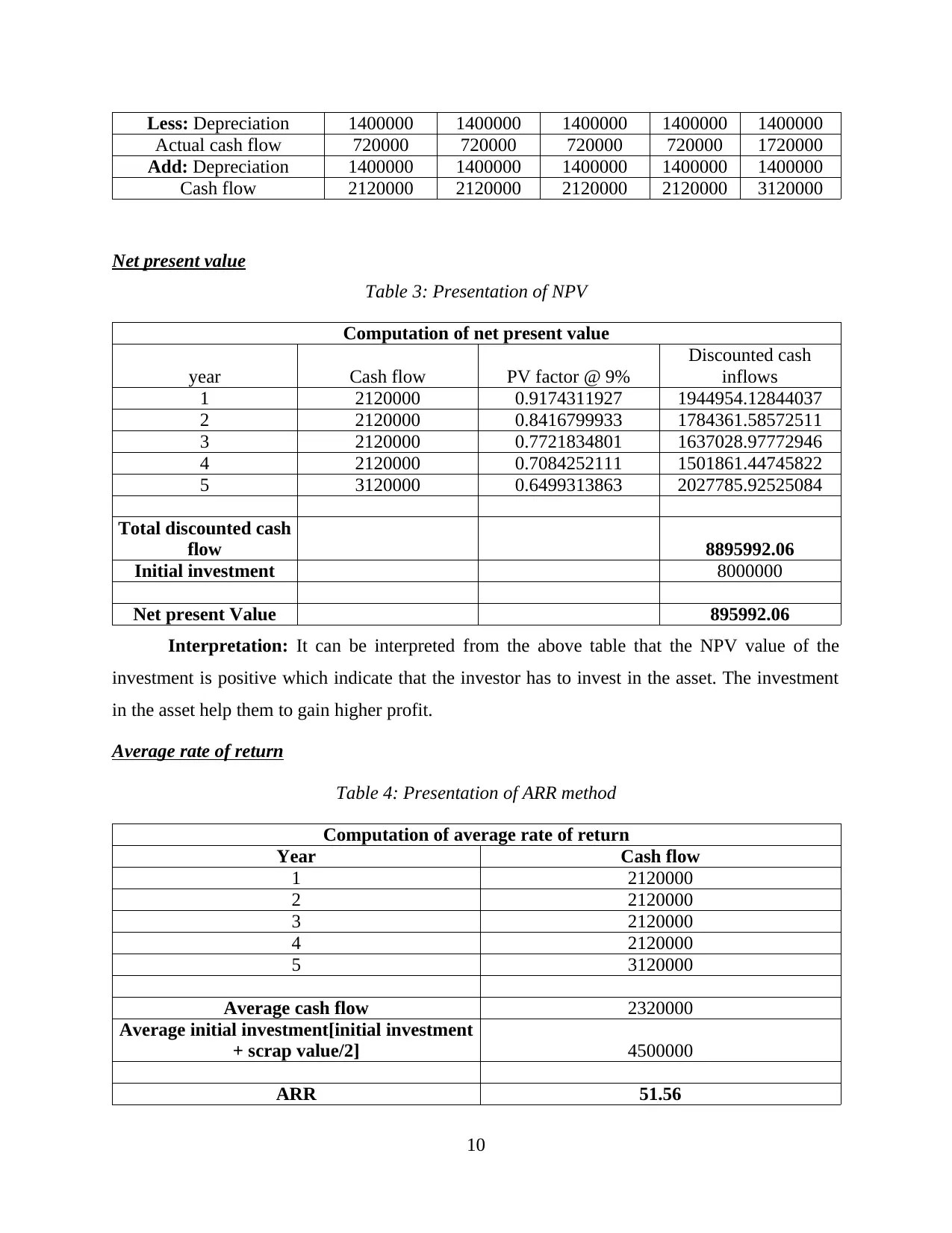
Less: Depreciation 1400000 1400000 1400000 1400000 1400000
Actual cash flow 720000 720000 720000 720000 1720000
Add: Depreciation 1400000 1400000 1400000 1400000 1400000
Cash flow 2120000 2120000 2120000 2120000 3120000
Net present value
Table 3: Presentation of NPV
Computation of net present value
year Cash flow PV factor @ 9%
Discounted cash
inflows
1 2120000 0.9174311927 1944954.12844037
2 2120000 0.8416799933 1784361.58572511
3 2120000 0.7721834801 1637028.97772946
4 2120000 0.7084252111 1501861.44745822
5 3120000 0.6499313863 2027785.92525084
Total discounted cash
flow 8895992.06
Initial investment 8000000
Net present Value 895992.06
Interpretation: It can be interpreted from the above table that the NPV value of the
investment is positive which indicate that the investor has to invest in the asset. The investment
in the asset help them to gain higher profit.
Average rate of return
Table 4: Presentation of ARR method
Computation of average rate of return
Year Cash flow
1 2120000
2 2120000
3 2120000
4 2120000
5 3120000
Average cash flow 2320000
Average initial investment[initial investment
+ scrap value/2] 4500000
ARR 51.56
10
⊘ This is a preview!⊘
Do you want full access?
Subscribe today to unlock all pages.
Trusted by 1+ million students worldwide
1 out of 17
Related Documents


Your All-in-One AI-Powered Toolkit for Academic Success.
+13062052269
info@desklib.com
Available 24*7 on WhatsApp / Email
![[object Object]](/_next/static/media/star-bottom.7253800d.svg)
Unlock your academic potential
Copyright © 2020–2026 A2Z Services. All Rights Reserved. Developed and managed by ZUCOL.