Financial Statistics Analysis of Hardware and Garden Supplies Sales
VerifiedAdded on 2020/05/08
|19
|2553
|358
Report
AI Summary
This report presents a financial statistics analysis of office supply sales data from Hardware and Garden Supplies. The analysis, based on a sample of 60 orders, explores various aspects including order priority, quantity, shipping costs, and customer segments. Descriptive statistics reveal trends in order frequency, sales, and shipping modes. Confidence intervals are calculated for sales and shipping costs, providing insights into the average values. Hypothesis testing examines relationships between shipping costs and order priority, as well as sales differences between regions. Correlation and regression analysis explores the relationship between order quantity and sales, showing a weak, positive, and linear correlation. The report concludes by highlighting key findings, limitations, and potential areas for further investigation, such as the impact of a larger sample size. The analysis uses statistical methods to provide a comprehensive overview of the sales data, including graphical representations to visualize key trends.
Running head: FINANCIAL STATISTICS
Financial Statistics
Name of the student
Name of the university
Author’s note
Financial Statistics
Name of the student
Name of the university
Author’s note
Paraphrase This Document
Need a fresh take? Get an instant paraphrase of this document with our AI Paraphraser
1FINANCIAL STATISTICS
Executive Summary
Herein, we present the analysis of office supply sales of Hardware and Garden Supplies.
The analysis of the data provided by the organization shows that with increase in shipping costs
as well as sales the number of orders decreases. The investigation shows that the orders have
diverse consumer segments, shipping modes and priority levels. There is no difference in the
shipping costs of critical and low priority orders. Moreover, there is no difference in the sales
from eastern and western region. The investigation shows that most of the orders are shipped
within 2 days of the orders being booked. Moreover, most of the orders for office supplies have a
critical priority. In addition, most of the orders are shipped through regular air and are from the
eastern region. The investigation shows that the highest number of customers is corporate
customers and the least number are consumer. We also find that there is a weak relationship
between order quantity and sales.
2FINANCIAL STATISTICS
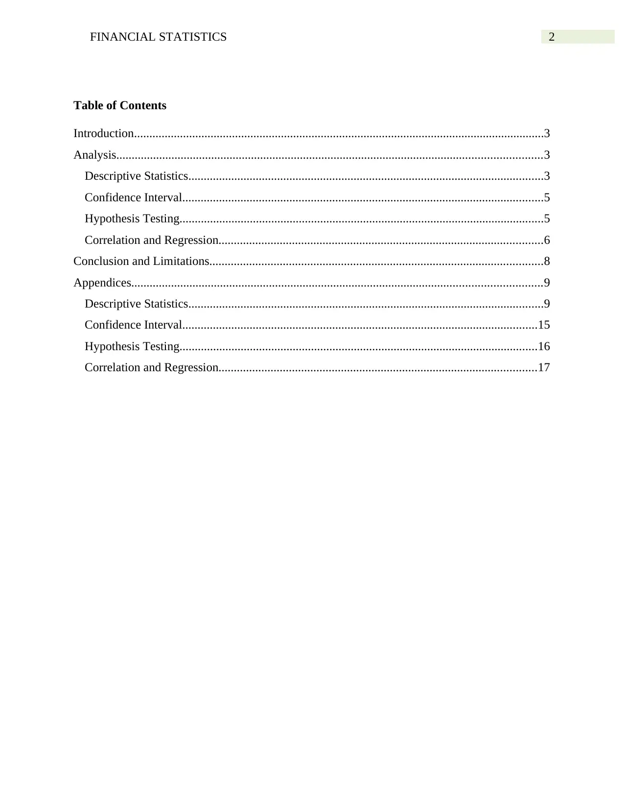
Table of Contents
Introduction......................................................................................................................................3
Analysis...........................................................................................................................................3
Descriptive Statistics....................................................................................................................3
Confidence Interval......................................................................................................................5
Hypothesis Testing.......................................................................................................................5
Correlation and Regression..........................................................................................................6
Conclusion and Limitations.............................................................................................................8
Appendices......................................................................................................................................9
Descriptive Statistics....................................................................................................................9
Confidence Interval....................................................................................................................15
Hypothesis Testing.....................................................................................................................16
Correlation and Regression........................................................................................................17
⊘ This is a preview!⊘
Do you want full access?
Subscribe today to unlock all pages.
Trusted by 1+ million students worldwide
3FINANCIAL STATISTICS
Introduction
In this assignment, we have analysed the office supply sales data provided by Hardware
and Garden Supplies The organization has provided information of office supplies for 2002
orders. For simplicity of calculation 60 orders randomly selected were analysed. Office supplies
data has provided information on different attributes. The various attributes for which
information is provided is order quantity, shipping costs as well as sales ($). Information
regarding the region from which the orders were generated, shipping mode along with the type of
customers and shipping priority was also provided. In this assignment, we have also compared
the sales for home office customers with all the customers. In addition, we have also compared
the shipping costs for the sample customers with the data of all the customers. The average
shipping costs for critical and low priority orders have been compared. The average sales for
orders from eastern and western region have also been compared. We have also examined the
relationship between order quantity and sales.
Analysis
Descriptive Statistics
Order ID
The variable represents a value through which the order can be tracked.
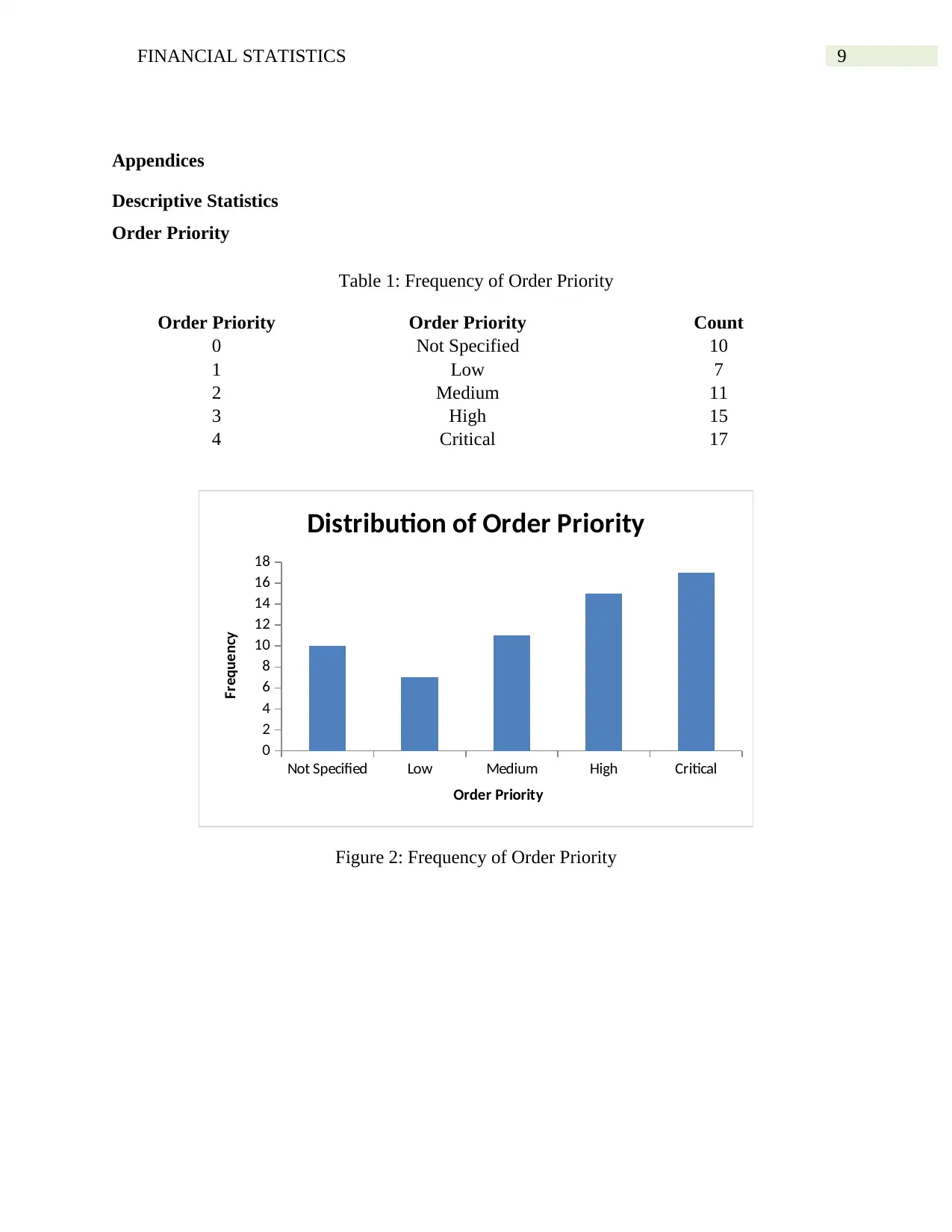
Order Priority
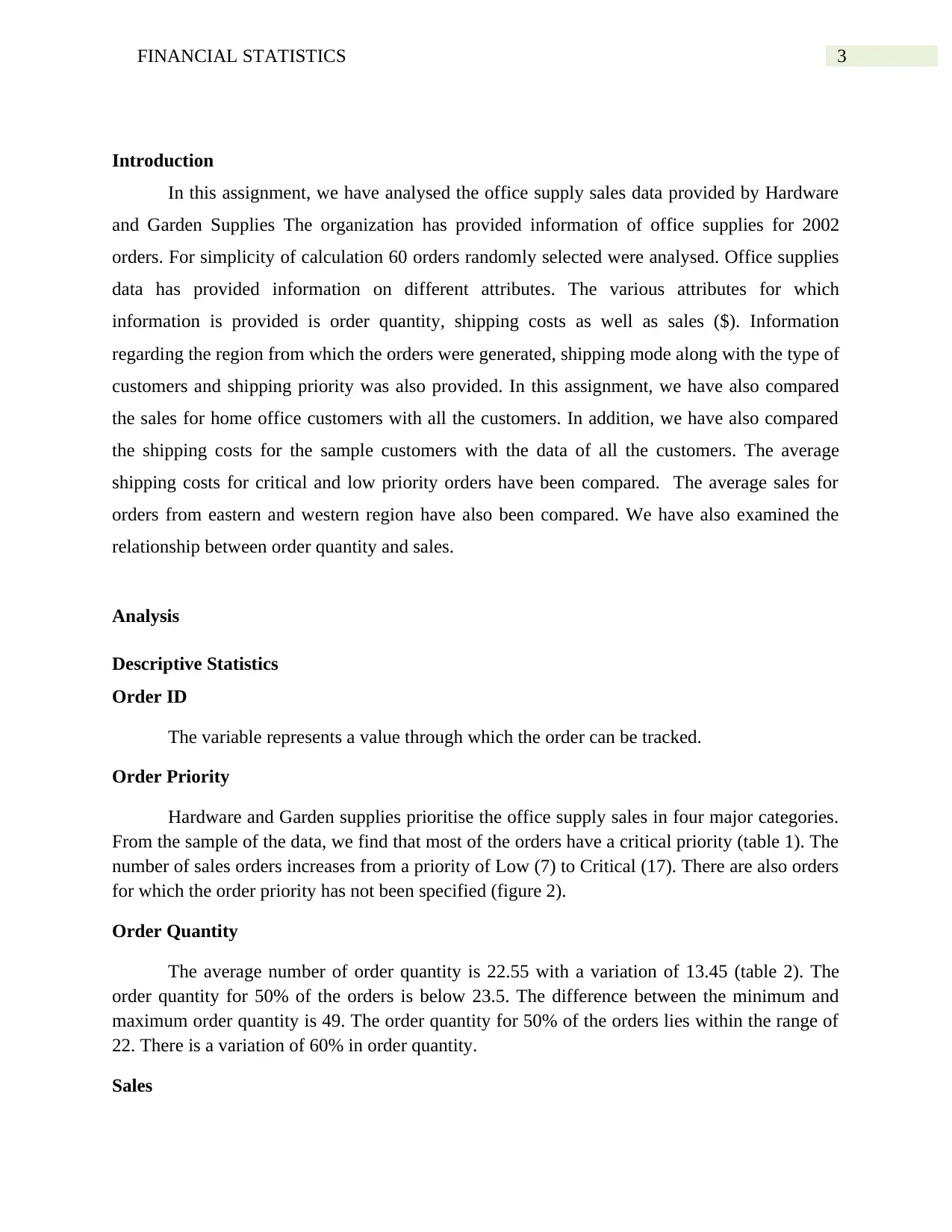
Hardware and Garden supplies prioritise the office supply sales in four major categories.
From the sample of the data, we find that most of the orders have a critical priority (table 1). The
number of sales orders increases from a priority of Low (7) to Critical (17). There are also orders
for which the order priority has not been specified (figure 2).
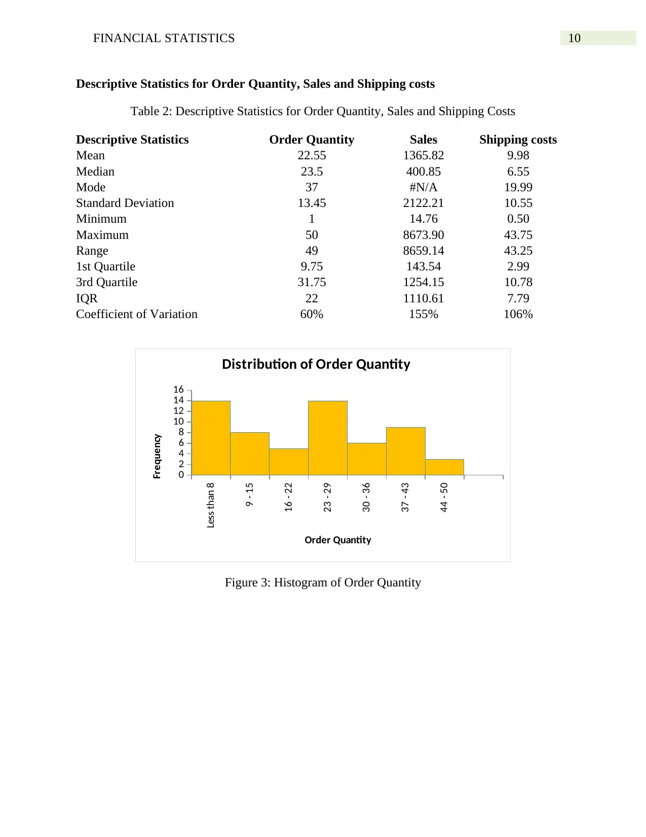
Order Quantity
The average number of order quantity is 22.55 with a variation of 13.45 (table 2). The
order quantity for 50% of the orders is below 23.5. The difference between the minimum and
maximum order quantity is 49. The order quantity for 50% of the orders lies within the range of
22. There is a variation of 60% in order quantity.
Sales
Introduction
In this assignment, we have analysed the office supply sales data provided by Hardware
and Garden Supplies The organization has provided information of office supplies for 2002
orders. For simplicity of calculation 60 orders randomly selected were analysed. Office supplies
data has provided information on different attributes. The various attributes for which
information is provided is order quantity, shipping costs as well as sales ($). Information
regarding the region from which the orders were generated, shipping mode along with the type of
customers and shipping priority was also provided. In this assignment, we have also compared
the sales for home office customers with all the customers. In addition, we have also compared
the shipping costs for the sample customers with the data of all the customers. The average
shipping costs for critical and low priority orders have been compared. The average sales for
orders from eastern and western region have also been compared. We have also examined the
relationship between order quantity and sales.
Analysis
Descriptive Statistics
Order ID
The variable represents a value through which the order can be tracked.
Order Priority
Hardware and Garden supplies prioritise the office supply sales in four major categories.
From the sample of the data, we find that most of the orders have a critical priority (table 1). The
number of sales orders increases from a priority of Low (7) to Critical (17). There are also orders
for which the order priority has not been specified (figure 2).
Order Quantity
The average number of order quantity is 22.55 with a variation of 13.45 (table 2). The
order quantity for 50% of the orders is below 23.5. The difference between the minimum and
maximum order quantity is 49. The order quantity for 50% of the orders lies within the range of
22. There is a variation of 60% in order quantity.
Sales
Paraphrase This Document
Need a fresh take? Get an instant paraphrase of this document with our AI Paraphraser
4FINANCIAL STATISTICS
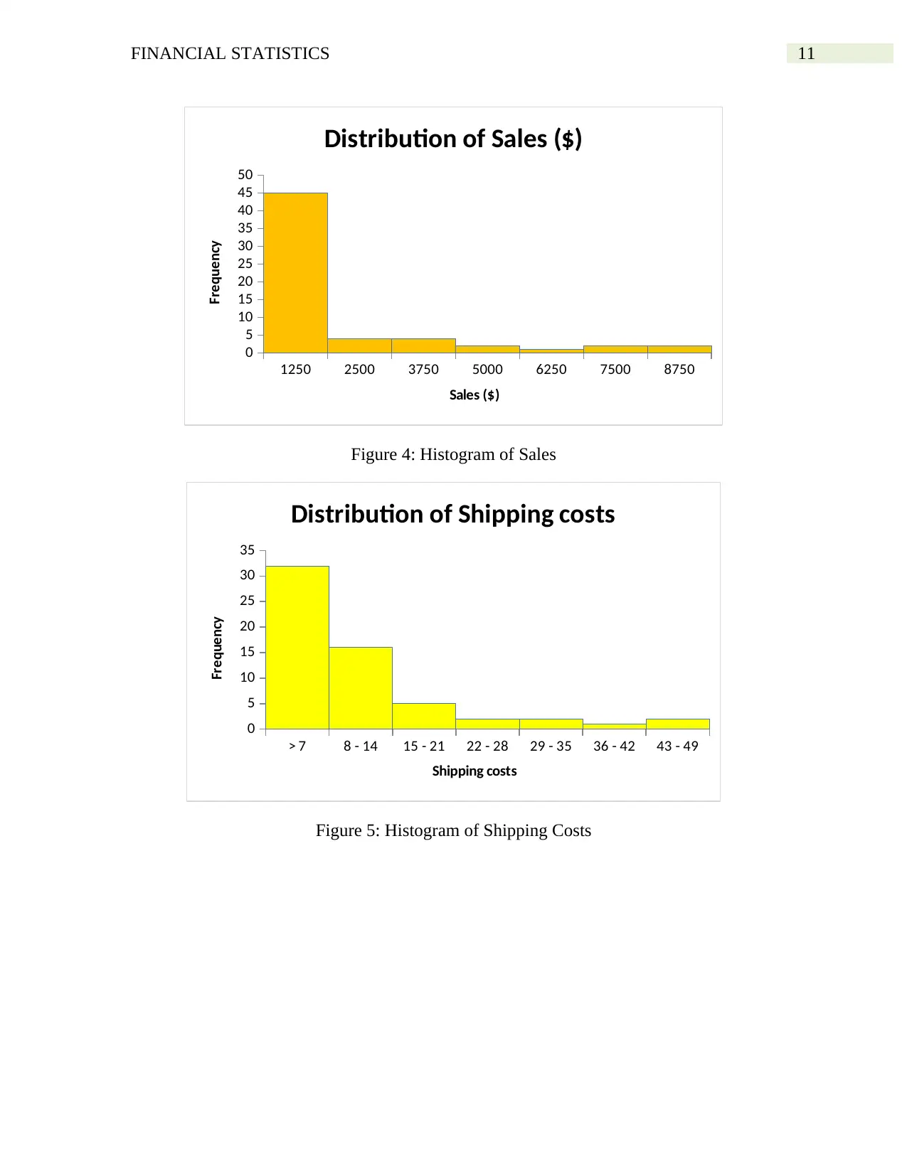
The average sales are $1365.82 with a variation of $2122.21. The sales for 50% of the
orders are below $400.85. The difference between the minimum and maximum sales is
$8659.14. The sales for 50% of the orders lie within a range of $1110.61. There is a variation of
155% in sales. The highest number of orders has sales of below $1250 (figure 4). With increase
in sales cost the frequency of orders decreases.
Ship Mode
Hardware and Garden supplies deliver office supplies in three shipping modes (table 3).
The sample data shows that most of the office supplies are delivered through Regular Air. The
least number of supplies are delivered through Delivery Truck (figure 6).
Shipping Cost
The cost of shipping the office supplies is provided in the data containing shipping costs
(table 2). The average shipping cost is $9.98 with a variation of $10.55. The shipping cost for
50% of the orders is below $6.55. The difference between the minimum and maximum
shipping costs is $43.25. The shipping costs for 50% of the orders lie within $7.79. There is a
variation of 106% in shipping costs. For most of the orders the shipping costs is below $7 (figure
5). As the shipping costs increases the frequency of order quantity decreases.
Region
Most of the office supplies for the organization are from the Eastern Region (table 4).
Hardware and Garden supplies also supply office sales goods to the western region (figure 7).
Customer Segment
The analysis of the data shows that there are four types of customers for Hardware and
Garden supplies. Most of the customers of the organization are corporate customers, closely
followed by Home office customers (table 5). The least number of customers are consumers
(figure 8).
Days to ship
The organization has provided information on “days to ship” for office supply products
(table 6). The analysis of the sample data shows that most of the office supplies would be
shipped in 1 or 2 days. Some of the orders are shipped on the very day they are booked
However, few of the orders are shipped in 3, 4 or even 7 days (figure 9). Moreover, no order is
shipped on the 5th or 6th day from which it is booked.
5FINANCIAL STATISTICS
Confidence Interval
Confidence Interval 1
We are 95% confident that the average sales amount of Home office customers lies
within the limits $971.03 and $1977.08. The average sales amount for Home office customers is
$1474.06. Thus, when a repeat sample of 60 customers is selected then the average sales amount
would lie within $971.03 and $1977.08 (table 7).
The mean sales for the total 2002 customers is $1716.69 (table 7). Thus, we find that the
average sales of the data of office supplies lies within the upper and lower limits of the sales data
for home office customers.
Confidence Interval 2
We are 95% confident that the average shipping costs of the sample of 60 customers lies
within the limits $7.31 and $12.65. The average shipping costs of 60 customers is $9.98. This,
can be interpreted as, when a repeat sample of 60 customers is selected then the average shipping
costs would lie within $7.31 and $12.65 (table 8).
The mean shipping costs for the total 2002 customers is $12.45 (table 8). Thus, we find
that the average shipping costs of office supplies lies within the upper and lower limits of the
shipping costs of the sample of 60 customers.
Hypothesis Testing
Hypothesis 1
In order to test the hypothesis that the shipping costs for orders having “Critical” priority
is higher than order having “Low” priority the two-sample t-test assuming equal variances is
used. The test result is presented in table 9. There are statistically no significant differences
between the shipping costs of “critical” and “low” priority orders, t(22) = 0.5737, p-value
=0.5720.
The mean shipping costs for critical and low priority orders are $11.93 and $8.82
respectively.
⊘ This is a preview!⊘
Do you want full access?
Subscribe today to unlock all pages.
Trusted by 1+ million students worldwide
6FINANCIAL STATISTICS
Hypothesis 2
In order to test the hypothesis that the average sales orders for orders from “Eastern”
region is different than orders from “Western” the two-sample t-test assuming equal variances is
used. The test results are presented in table 10. There are statistically no significant differences
in the average sales orders between “Eastern” and “Western” region, t(58) = 1.354, p-value
=0.181.
The mean sales orders for Eastern and Western region are $1666.54 and $914.73
respectively.
Correlation and Regression
Correlation
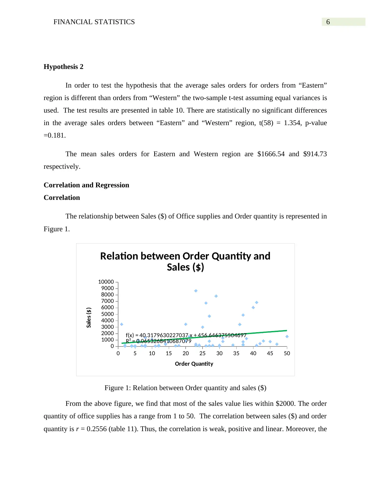
The relationship between Sales ($) of Office supplies and Order quantity is represented in
Figure 1.
0 5 10 15 20 25 30 35 40 45 50
0
1000
2000
3000
4000
5000
6000
7000
8000
9000
10000
f(x) = 40.3179630227037 x + 456.646375504697
R² = 0.0653268410687079
Relation between Order Quantity and
Sales ($)
Order Quantity
Sales ($)
Figure 1: Relation between Order quantity and sales ($)
From the above figure, we find that most of the sales value lies within $2000. The order
quantity of office supplies has a range from 1 to 50. The correlation between sales ($) and order
quantity is r = 0.2556 (table 11). Thus, the correlation is weak, positive and linear. Moreover, the
Hypothesis 2
In order to test the hypothesis that the average sales orders for orders from “Eastern”
region is different than orders from “Western” the two-sample t-test assuming equal variances is
used. The test results are presented in table 10. There are statistically no significant differences
in the average sales orders between “Eastern” and “Western” region, t(58) = 1.354, p-value
=0.181.
The mean sales orders for Eastern and Western region are $1666.54 and $914.73
respectively.
Correlation and Regression
Correlation
The relationship between Sales ($) of Office supplies and Order quantity is represented in
Figure 1.
0 5 10 15 20 25 30 35 40 45 50
0
1000
2000
3000
4000
5000
6000
7000
8000
9000
10000
f(x) = 40.3179630227037 x + 456.646375504697
R² = 0.0653268410687079
Relation between Order Quantity and
Sales ($)
Order Quantity
Sales ($)
Figure 1: Relation between Order quantity and sales ($)
From the above figure, we find that most of the sales value lies within $2000. The order
quantity of office supplies has a range from 1 to 50. The correlation between sales ($) and order
quantity is r = 0.2556 (table 11). Thus, the correlation is weak, positive and linear. Moreover, the
Paraphrase This Document
Need a fresh take? Get an instant paraphrase of this document with our AI Paraphraser
7FINANCIAL STATISTICS
coefficient of determination R2 = 0.0653. Thus 6.53% of the variability in Sales ($) can be
predicted from R2.
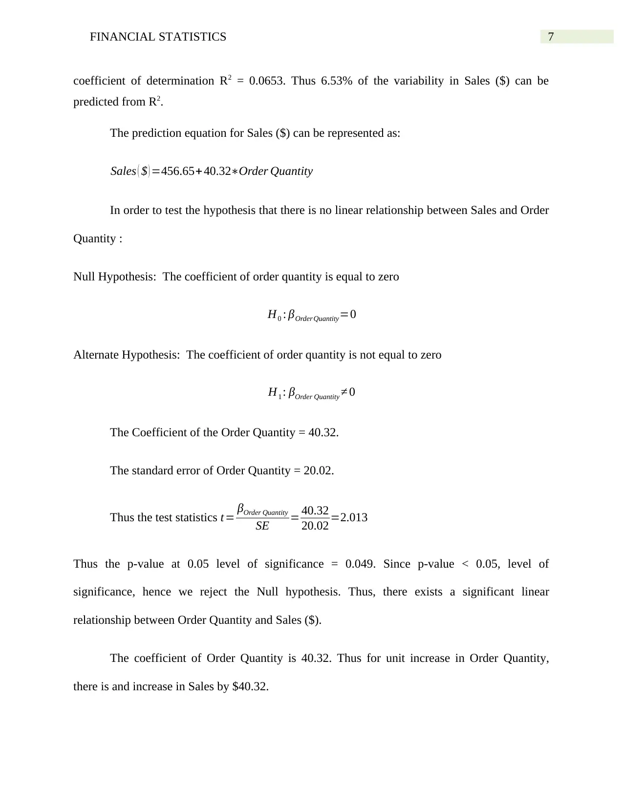
The prediction equation for Sales ($) can be represented as:
Sales ( $ ) =456.65+ 40.32∗Order Quantity
In order to test the hypothesis that there is no linear relationship between Sales and Order
Quantity :
Null Hypothesis: The coefficient of order quantity is equal to zero
H0 : βOrder Quantity=0
Alternate Hypothesis: The coefficient of order quantity is not equal to zero
H1 : βOrder Quantity ≠ 0
The Coefficient of the Order Quantity = 40.32.
The standard error of Order Quantity = 20.02.
Thus the test statistics t= βOrder Quantity
SE = 40.32
20.02 =2.013
Thus the p-value at 0.05 level of significance = 0.049. Since p-value < 0.05, level of
significance, hence we reject the Null hypothesis. Thus, there exists a significant linear
relationship between Order Quantity and Sales ($).
The coefficient of Order Quantity is 40.32. Thus for unit increase in Order Quantity,
there is and increase in Sales by $40.32.
coefficient of determination R2 = 0.0653. Thus 6.53% of the variability in Sales ($) can be
predicted from R2.
The prediction equation for Sales ($) can be represented as:
Sales ( $ ) =456.65+ 40.32∗Order Quantity
In order to test the hypothesis that there is no linear relationship between Sales and Order
Quantity :
Null Hypothesis: The coefficient of order quantity is equal to zero
H0 : βOrder Quantity=0
Alternate Hypothesis: The coefficient of order quantity is not equal to zero
H1 : βOrder Quantity ≠ 0
The Coefficient of the Order Quantity = 40.32.
The standard error of Order Quantity = 20.02.
Thus the test statistics t= βOrder Quantity
SE = 40.32
20.02 =2.013
Thus the p-value at 0.05 level of significance = 0.049. Since p-value < 0.05, level of
significance, hence we reject the Null hypothesis. Thus, there exists a significant linear
relationship between Order Quantity and Sales ($).
The coefficient of Order Quantity is 40.32. Thus for unit increase in Order Quantity,
there is and increase in Sales by $40.32.
8FINANCIAL STATISTICS
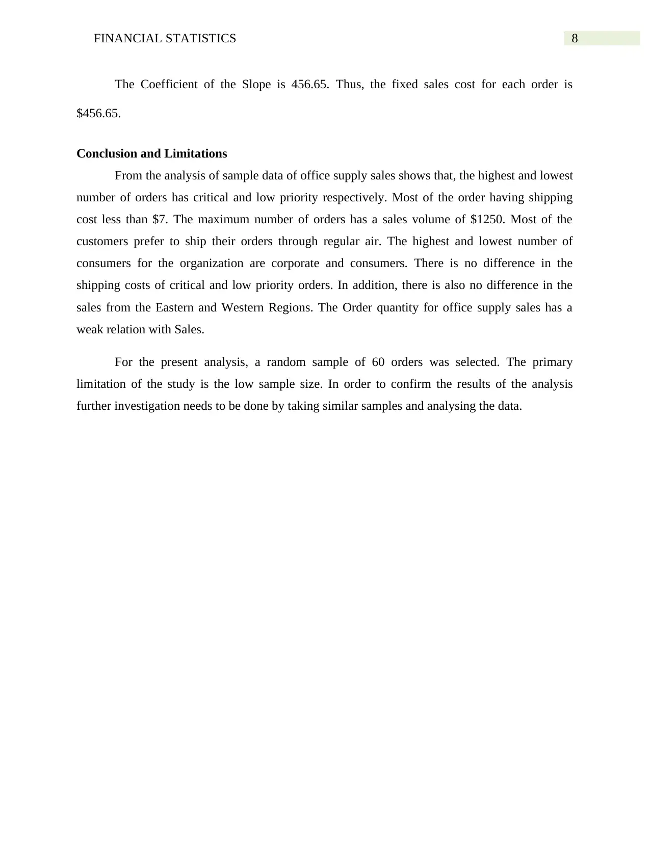
The Coefficient of the Slope is 456.65. Thus, the fixed sales cost for each order is
$456.65.
Conclusion and Limitations
From the analysis of sample data of office supply sales shows that, the highest and lowest
number of orders has critical and low priority respectively. Most of the order having shipping
cost less than $7. The maximum number of orders has a sales volume of $1250. Most of the
customers prefer to ship their orders through regular air. The highest and lowest number of
consumers for the organization are corporate and consumers. There is no difference in the
shipping costs of critical and low priority orders. In addition, there is also no difference in the
sales from the Eastern and Western Regions. The Order quantity for office supply sales has a
weak relation with Sales.
For the present analysis, a random sample of 60 orders was selected. The primary
limitation of the study is the low sample size. In order to confirm the results of the analysis
further investigation needs to be done by taking similar samples and analysing the data.
⊘ This is a preview!⊘
Do you want full access?
Subscribe today to unlock all pages.
Trusted by 1+ million students worldwide
9FINANCIAL STATISTICS
Appendices
Descriptive Statistics
Order Priority
Table 1: Frequency of Order Priority
Order Priority Order Priority Count
0 Not Specified 10
1 Low 7
2 Medium 11
3 High 15
4 Critical 17
Not Specified Low Medium High Critical
0
2
4
6
8
10
12
14
16
18
Distribution of Order Priority
Order Priority
Frequency
Figure 2: Frequency of Order Priority
Paraphrase This Document
Need a fresh take? Get an instant paraphrase of this document with our AI Paraphraser
10FINANCIAL STATISTICS
Descriptive Statistics for Order Quantity, Sales and Shipping costs
Table 2: Descriptive Statistics for Order Quantity, Sales and Shipping Costs
Descriptive Statistics Order Quantity Sales Shipping costs
Mean 22.55 1365.82 9.98
Median 23.5 400.85 6.55
Mode 37 #N/A 19.99
Standard Deviation 13.45 2122.21 10.55
Minimum 1 14.76 0.50
Maximum 50 8673.90 43.75
Range 49 8659.14 43.25
1st Quartile 9.75 143.54 2.99
3rd Quartile 31.75 1254.15 10.78
IQR 22 1110.61 7.79
Coefficient of Variation 60% 155% 106%
Less than 8
9 - 15
16 - 22
23 - 29
30 - 36
37 - 43
44 - 500
2
4
6
8
10
12
14
16
Distribution of Order Quantity
Order Quantity
Frequency
Figure 3: Histogram of Order Quantity
11FINANCIAL STATISTICS
1250 2500 3750 5000 6250 7500 8750
0
5
10
15
20
25
30
35
40
45
50
Distribution of Sales ($)
Sales ($)
Frequency
Figure 4: Histogram of Sales
> 7 8 - 14 15 - 21 22 - 28 29 - 35 36 - 42 43 - 49
0
5
10
15
20
25
30
35
Distribution of Shipping costs
Shipping costs
Frequency
Figure 5: Histogram of Shipping Costs
⊘ This is a preview!⊘
Do you want full access?
Subscribe today to unlock all pages.
Trusted by 1+ million students worldwide
1 out of 19
Related Documents


Your All-in-One AI-Powered Toolkit for Academic Success.
+13062052269
info@desklib.com
Available 24*7 on WhatsApp / Email
![[object Object]](/_next/static/media/star-bottom.7253800d.svg)
Unlock your academic potential
Copyright © 2020–2026 A2Z Services. All Rights Reserved. Developed and managed by ZUCOL.