Financial Statistics Report: Analysis of Movie Purchase Data
VerifiedAdded on 2023/06/05
|22
|4691
|75
Report
AI Summary
This report presents a comprehensive analysis of financial statistics, focusing on the application of statistical tools to understand and interpret data related to movie purchases. The report begins with an executive summary highlighting the importance of statistics in business decision-making and data analysis. It then delves into various statistical methods, including VLOOKUP and INDEX functions for random sampling, and provides summary statistics such as mean, median, and standard deviation. The analysis extends to frequency tables, histograms, and pie charts to visualize age-wise purchase patterns and expenditure by movie genre. Confidence intervals are calculated to assess the reliability of sample data. The report also includes hypothesis testing to determine the significance of the findings. The report's conclusions offer valuable insights into consumer behavior, preferences, and potential strategies for maximizing profitability based on the statistical analysis of historical data.
Question and Answer
1 | P a g e
Financial Statistics
1 | P a g e
Financial Statistics
Paraphrase This Document
Need a fresh take? Get an instant paraphrase of this document with our AI Paraphraser
Question and Answer
Executive Summary
There is no corner left, where use of statistics is negligible in business area, whether it is decision
making, or providing treat to their client, all comes under controlled calculated expense, so that it
cannot hamper the profit of business and, the hero is statistics which guide all the processes from
background. In this report we have tried to show that how we can retrieve the useful information
from given chunk of data. To process the data, into useful information, we have so used several
tools and table so that, we can easily grab the useful information which is hidden behind this
data. Further, the in-depth use of statistical tools shows that what can be out future direction
based on historical data and relationship with future.
2 | P a g e
Question and Answer
Contents
Solution 1.........................................................................................................................................4
Solution 2.........................................................................................................................................4
Solution 2(1)................................................................................................................................6
Solution 2(ii)................................................................................................................................7
Solution 2(iii)...............................................................................................................................7
Solution 3.........................................................................................................................................8
Solution 3(a)................................................................................................................................8
Solution 4.......................................................................................................................................10
Solution 4(1)..............................................................................................................................10
Solution 4(2)..............................................................................................................................11
Solution 5.......................................................................................................................................11
Solution 5(i)...............................................................................................................................12
Solution 5(ii)..............................................................................................................................12
Solution 5(iii).............................................................................................................................13
Solution 5(iv).............................................................................................................................13
Solution 6.......................................................................................................................................14
3 | P a g e
⊘ This is a preview!⊘
Do you want full access?
Subscribe today to unlock all pages.
Trusted by 1+ million students worldwide
Question and Answer
Solution 1
The first method of selecting random sample, we have used VLOOKUP function of excel for
selecting the random sample in this case, The VLOOUP function extract the data on given
criteria =VLOOKUP (Lookup value, table array, column index number, false), the false value
extract if there is exact match. Th use of VLOOKUP function is more useful in extracting data
from given references, and very useful tools in analysis when data extraction from database is
tedious task.
The second method, the random sample is extracted by index function, INDEX (array,
RANDBETWEEN (array)), column number), from this function we can extract the random
number in given data. The combination of INDEX and RANDBETWEEN function provide the
best random variable, but we must keep in mind that this variable is very susceptible to change,
even, minute change in column also results variation in processed data and cause problem. So
during analysis we must copy first the extracted data and then analyse, so that it cannot be
changed later.
Solution 2
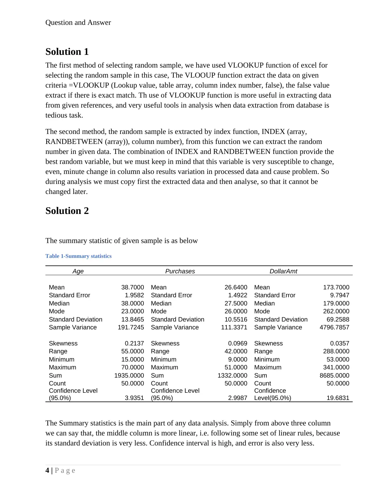
The summary statistic of given sample is as below
Table 1-Summary statistics
Age Purchases DollarAmt
Mean 38.7000 Mean 26.6400 Mean 173.7000
Standard Error 1.9582 Standard Error 1.4922 Standard Error 9.7947
Median 38.0000 Median 27.5000 Median 179.0000
Mode 23.0000 Mode 26.0000 Mode 262.0000
Standard Deviation 13.8465 Standard Deviation 10.5516 Standard Deviation 69.2588
Sample Variance 191.7245 Sample Variance 111.3371 Sample Variance 4796.7857
Skewness 0.2137 Skewness 0.0969 Skewness 0.0357
Range 55.0000 Range 42.0000 Range 288.0000
Minimum 15.0000 Minimum 9.0000 Minimum 53.0000
Maximum 70.0000 Maximum 51.0000 Maximum 341.0000
Sum 1935.0000 Sum 1332.0000 Sum 8685.0000
Count 50.0000 Count 50.0000 Count 50.0000
Confidence Level
(95.0%) 3.9351
Confidence Level
(95.0%) 2.9987
Confidence
Level(95.0%) 19.6831
The Summary statistics is the main part of any data analysis. Simply from above three column
we can say that, the middle column is more linear, i.e. following some set of linear rules, because
its standard deviation is very less. Confidence interval is high, and error is also very less.
4 | P a g e
Solution 1
The first method of selecting random sample, we have used VLOOKUP function of excel for
selecting the random sample in this case, The VLOOUP function extract the data on given
criteria =VLOOKUP (Lookup value, table array, column index number, false), the false value
extract if there is exact match. Th use of VLOOKUP function is more useful in extracting data
from given references, and very useful tools in analysis when data extraction from database is
tedious task.
The second method, the random sample is extracted by index function, INDEX (array,
RANDBETWEEN (array)), column number), from this function we can extract the random
number in given data. The combination of INDEX and RANDBETWEEN function provide the
best random variable, but we must keep in mind that this variable is very susceptible to change,
even, minute change in column also results variation in processed data and cause problem. So
during analysis we must copy first the extracted data and then analyse, so that it cannot be
changed later.
Solution 2
The summary statistic of given sample is as below
Table 1-Summary statistics
Age Purchases DollarAmt
Mean 38.7000 Mean 26.6400 Mean 173.7000
Standard Error 1.9582 Standard Error 1.4922 Standard Error 9.7947
Median 38.0000 Median 27.5000 Median 179.0000
Mode 23.0000 Mode 26.0000 Mode 262.0000
Standard Deviation 13.8465 Standard Deviation 10.5516 Standard Deviation 69.2588
Sample Variance 191.7245 Sample Variance 111.3371 Sample Variance 4796.7857
Skewness 0.2137 Skewness 0.0969 Skewness 0.0357
Range 55.0000 Range 42.0000 Range 288.0000
Minimum 15.0000 Minimum 9.0000 Minimum 53.0000
Maximum 70.0000 Maximum 51.0000 Maximum 341.0000
Sum 1935.0000 Sum 1332.0000 Sum 8685.0000
Count 50.0000 Count 50.0000 Count 50.0000
Confidence Level
(95.0%) 3.9351
Confidence Level
(95.0%) 2.9987
Confidence
Level(95.0%) 19.6831
The Summary statistics is the main part of any data analysis. Simply from above three column
we can say that, the middle column is more linear, i.e. following some set of linear rules, because
its standard deviation is very less. Confidence interval is high, and error is also very less.
4 | P a g e
Paraphrase This Document
Need a fresh take? Get an instant paraphrase of this document with our AI Paraphraser
Question and Answer
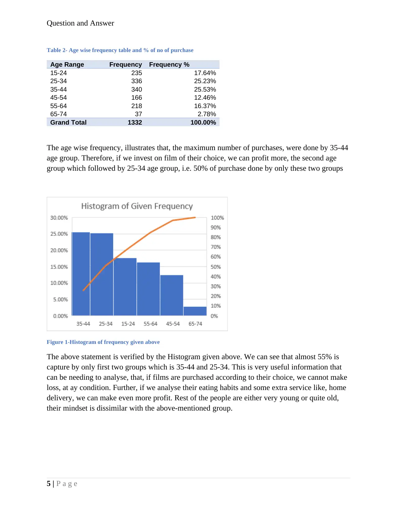
Table 2- Age wise frequency table and % of no of purchase
Age Range Frequency Frequency %
15-24 235 17.64%
25-34 336 25.23%
35-44 340 25.53%
45-54 166 12.46%
55-64 218 16.37%
65-74 37 2.78%
Grand Total 1332 100.00%
The age wise frequency, illustrates that, the maximum number of purchases, were done by 35-44
age group. Therefore, if we invest on film of their choice, we can profit more, the second age
group which followed by 25-34 age group, i.e. 50% of purchase done by only these two groups
Figure 1-Histogram of frequency given above
The above statement is verified by the Histogram given above. We can see that almost 55% is
capture by only first two groups which is 35-44 and 25-34. This is very useful information that
can be needing to analyse, that, if films are purchased according to their choice, we cannot make
loss, at ay condition. Further, if we analyse their eating habits and some extra service like, home
delivery, we can make even more profit. Rest of the people are either very young or quite old,
their mindset is dissimilar with the above-mentioned group.
5 | P a g e
Question and Answer
18%
25%
26%
12%
16% 3%
A e i e re enc Pie artg w s F qu y Ch
15-24
25-34
35-44
45-54
55-64
65-74
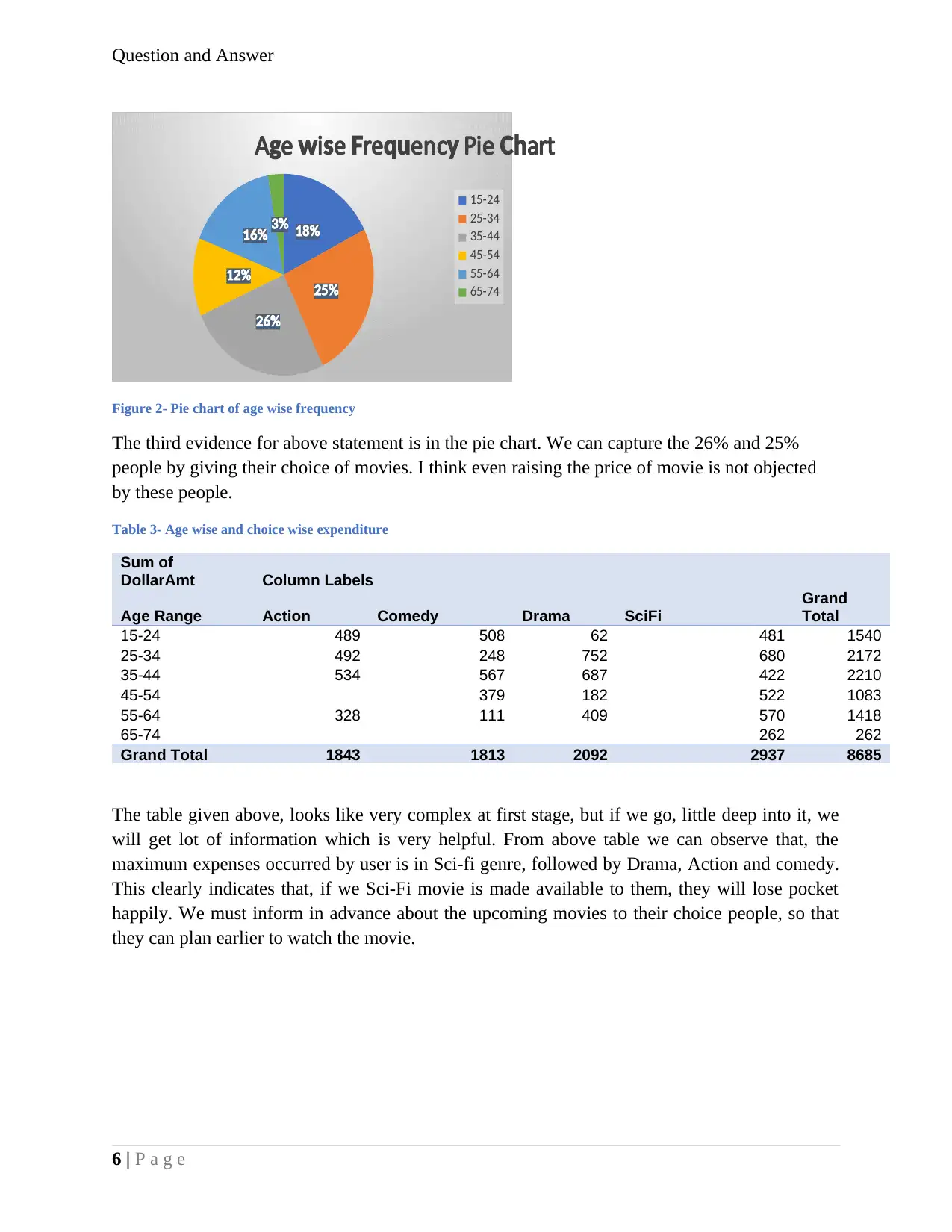
Figure 2- Pie chart of age wise frequency
The third evidence for above statement is in the pie chart. We can capture the 26% and 25%
people by giving their choice of movies. I think even raising the price of movie is not objected
by these people.
Table 3- Age wise and choice wise expenditure
Sum of
DollarAmt Column Labels
Age Range Action Comedy Drama SciFi
Grand
Total
15-24 489 508 62 481 1540
25-34 492 248 752 680 2172
35-44 534 567 687 422 2210
45-54 379 182 522 1083
55-64 328 111 409 570 1418
65-74 262 262
Grand Total 1843 1813 2092 2937 8685
The table given above, looks like very complex at first stage, but if we go, little deep into it, we
will get lot of information which is very helpful. From above table we can observe that, the
maximum expenses occurred by user is in Sci-fi genre, followed by Drama, Action and comedy.
This clearly indicates that, if we Sci-Fi movie is made available to them, they will lose pocket
happily. We must inform in advance about the upcoming movies to their choice people, so that
they can plan earlier to watch the movie.
6 | P a g e
18%
25%
26%
12%
16% 3%
A e i e re enc Pie artg w s F qu y Ch
15-24
25-34
35-44
45-54
55-64
65-74
Figure 2- Pie chart of age wise frequency
The third evidence for above statement is in the pie chart. We can capture the 26% and 25%
people by giving their choice of movies. I think even raising the price of movie is not objected
by these people.
Table 3- Age wise and choice wise expenditure
Sum of
DollarAmt Column Labels
Age Range Action Comedy Drama SciFi
Grand
Total
15-24 489 508 62 481 1540
25-34 492 248 752 680 2172
35-44 534 567 687 422 2210
45-54 379 182 522 1083
55-64 328 111 409 570 1418
65-74 262 262
Grand Total 1843 1813 2092 2937 8685
The table given above, looks like very complex at first stage, but if we go, little deep into it, we
will get lot of information which is very helpful. From above table we can observe that, the
maximum expenses occurred by user is in Sci-fi genre, followed by Drama, Action and comedy.
This clearly indicates that, if we Sci-Fi movie is made available to them, they will lose pocket
happily. We must inform in advance about the upcoming movies to their choice people, so that
they can plan earlier to watch the movie.
6 | P a g e
⊘ This is a preview!⊘
Do you want full access?
Subscribe today to unlock all pages.
Trusted by 1+ million students worldwide
Question and Answer
15-24 25-34 35-44 45-54 55-64 65-74
0
100
200
300
400
500
600
700
800
l tered c artC us h
Action
omedC y
ramaD
ci iS F
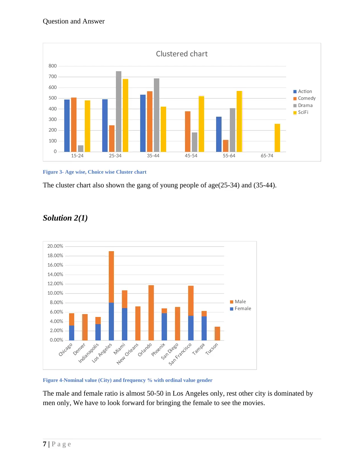
Figure 3- Age wise, Choice wise Cluster chart
The cluster chart also shown the gang of young people of age(25-34) and (35-44).
Solution 2(1)
ica oCh g
en erD v
ndianapoliI s
o An eleL s g s
Miami
e rleanN w O s
rlandoO
P oenih x
an ie oS D g
an ranci coS F s
Tampa
T c onu s
0.00%
2.00%
4.00%
6.00%
8.00%
10.00%
12.00%
14.00%
16.00%
18.00%
20.00%
Male
emaleF
Figure 4-Nominal value (City) and frequency % with ordinal value gender
The male and female ratio is almost 50-50 in Los Angeles only, rest other city is dominated by
men only, We have to look forward for bringing the female to see the movies.
7 | P a g e
15-24 25-34 35-44 45-54 55-64 65-74
0
100
200
300
400
500
600
700
800
l tered c artC us h
Action
omedC y
ramaD
ci iS F
Figure 3- Age wise, Choice wise Cluster chart
The cluster chart also shown the gang of young people of age(25-34) and (35-44).
Solution 2(1)
ica oCh g
en erD v
ndianapoliI s
o An eleL s g s
Miami
e rleanN w O s
rlandoO
P oenih x
an ie oS D g
an ranci coS F s
Tampa
T c onu s
0.00%
2.00%
4.00%
6.00%
8.00%
10.00%
12.00%
14.00%
16.00%
18.00%
20.00%
Male
emaleF
Figure 4-Nominal value (City) and frequency % with ordinal value gender
The male and female ratio is almost 50-50 in Los Angeles only, rest other city is dominated by
men only, We have to look forward for bringing the female to see the movies.
7 | P a g e
Paraphrase This Document
Need a fresh take? Get an instant paraphrase of this document with our AI Paraphraser
Question and Answer
Solution 2(ii)
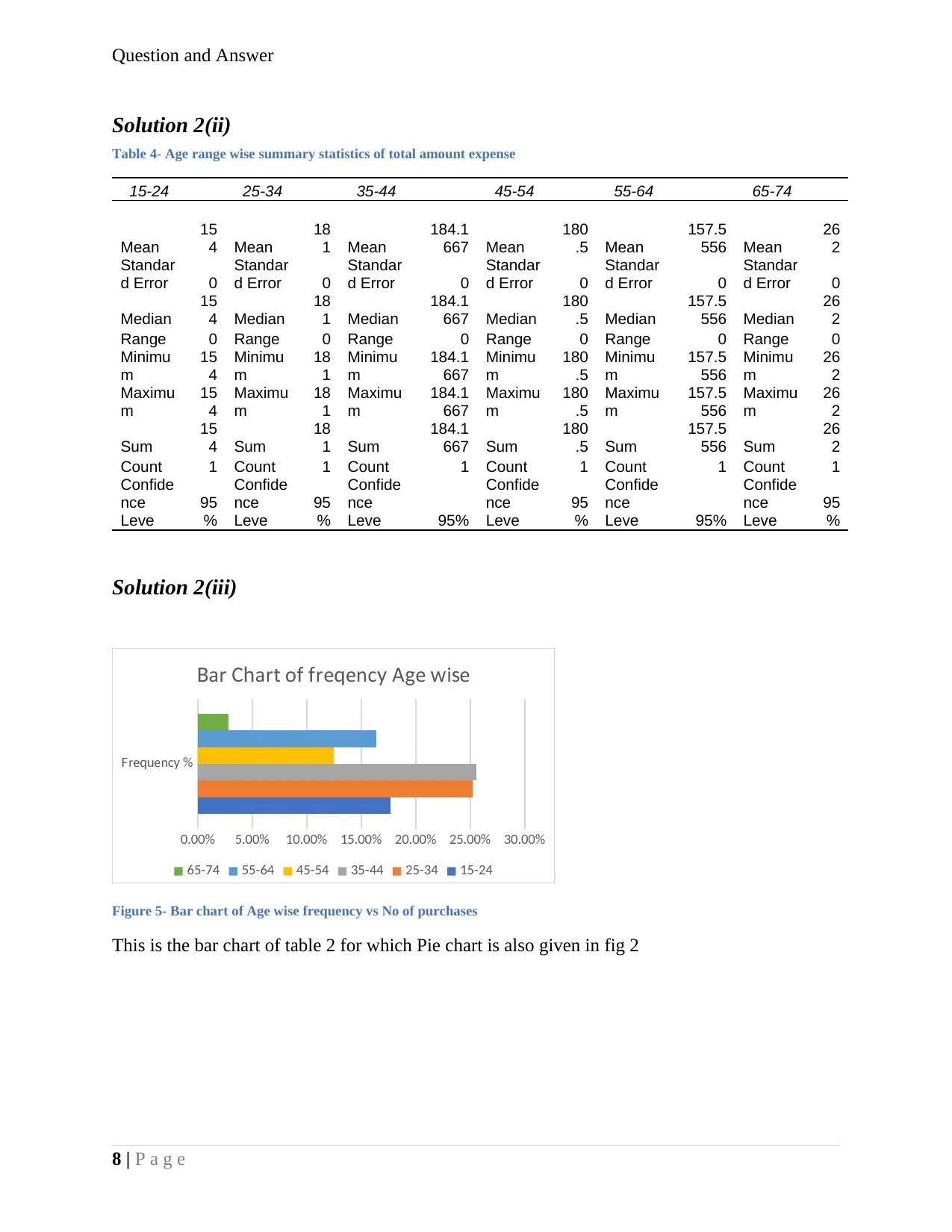
Table 4- Age range wise summary statistics of total amount expense
15-24 25-34 35-44 45-54 55-64 65-74
Mean
15
4 Mean
18
1 Mean
184.1
667 Mean
180
.5 Mean
157.5
556 Mean
26
2
Standar
d Error 0
Standar
d Error 0
Standar
d Error 0
Standar
d Error 0
Standar
d Error 0
Standar
d Error 0
Median
15
4 Median
18
1 Median
184.1
667 Median
180
.5 Median
157.5
556 Median
26
2
Range 0 Range 0 Range 0 Range 0 Range 0 Range 0
Minimu
m
15
4
Minimu
m
18
1
Minimu
m
184.1
667
Minimu
m
180
.5
Minimu
m
157.5
556
Minimu
m
26
2
Maximu
m
15
4
Maximu
m
18
1
Maximu
m
184.1
667
Maximu
m
180
.5
Maximu
m
157.5
556
Maximu
m
26
2
Sum
15
4 Sum
18
1 Sum
184.1
667 Sum
180
.5 Sum
157.5
556 Sum
26
2
Count 1 Count 1 Count 1 Count 1 Count 1 Count 1
Confide
nce
Leve
95
%
Confide
nce
Leve
95
%
Confide
nce
Leve 95%
Confide
nce
Leve
95
%
Confide
nce
Leve 95%
Confide
nce
Leve
95
%
Solution 2(iii)
re encF qu y %
0.00% 5.00% 10.00% 15.00% 20.00% 25.00% 30.00%
ar art o re enc A e i eB Ch f f q y g w s
65-74 55-64 45-54 35-44 25-34 15-24
Figure 5- Bar chart of Age wise frequency vs No of purchases
This is the bar chart of table 2 for which Pie chart is also given in fig 2
8 | P a g e
Solution 2(ii)
Table 4- Age range wise summary statistics of total amount expense
15-24 25-34 35-44 45-54 55-64 65-74
Mean
15
4 Mean
18
1 Mean
184.1
667 Mean
180
.5 Mean
157.5
556 Mean
26
2
Standar
d Error 0
Standar
d Error 0
Standar
d Error 0
Standar
d Error 0
Standar
d Error 0
Standar
d Error 0
Median
15
4 Median
18
1 Median
184.1
667 Median
180
.5 Median
157.5
556 Median
26
2
Range 0 Range 0 Range 0 Range 0 Range 0 Range 0
Minimu
m
15
4
Minimu
m
18
1
Minimu
m
184.1
667
Minimu
m
180
.5
Minimu
m
157.5
556
Minimu
m
26
2
Maximu
m
15
4
Maximu
m
18
1
Maximu
m
184.1
667
Maximu
m
180
.5
Maximu
m
157.5
556
Maximu
m
26
2
Sum
15
4 Sum
18
1 Sum
184.1
667 Sum
180
.5 Sum
157.5
556 Sum
26
2
Count 1 Count 1 Count 1 Count 1 Count 1 Count 1
Confide
nce
Leve
95
%
Confide
nce
Leve
95
%
Confide
nce
Leve 95%
Confide
nce
Leve
95
%
Confide
nce
Leve 95%
Confide
nce
Leve
95
%
Solution 2(iii)
re encF qu y %
0.00% 5.00% 10.00% 15.00% 20.00% 25.00% 30.00%
ar art o re enc A e i eB Ch f f q y g w s
65-74 55-64 45-54 35-44 25-34 15-24
Figure 5- Bar chart of Age wise frequency vs No of purchases
This is the bar chart of table 2 for which Pie chart is also given in fig 2
8 | P a g e
Question and Answer
0-14 15-24 25-34 35-44 45-54 55-64 65-74 75-84
0
500
1000
1500
2000
2500
re nc Pol on o A e an e ollarF qu y yg f g R g Vs D
Amo ntu
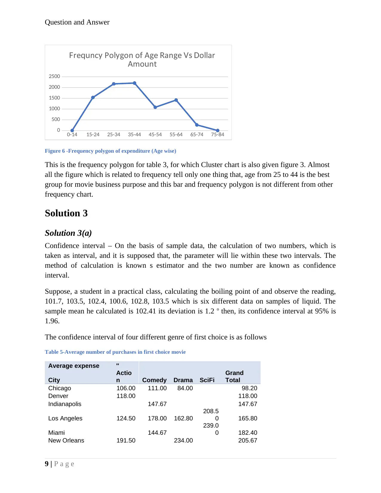
Figure 6 -Frequency polygon of expenditure (Age wise)
This is the frequency polygon for table 3, for which Cluster chart is also given figure 3. Almost
all the figure which is related to frequency tell only one thing that, age from 25 to 44 is the best
group for movie business purpose and this bar and frequency polygon is not different from other
frequency chart.
Solution 3
Solution 3(a)
Confidence interval – On the basis of sample data, the calculation of two numbers, which is
taken as interval, and it is supposed that, the parameter will lie within these two intervals. The
method of calculation is known s estimator and the two number are known as confidence
interval.
Suppose, a student in a practical class, calculating the boiling point of and observe the reading,
101.7, 103.5, 102.4, 100.6, 102.8, 103.5 which is six different data on samples of liquid. The
sample mean he calculated is 102.41 its deviation is 1.2 o then, its confidence interval at 95% is
1.96.
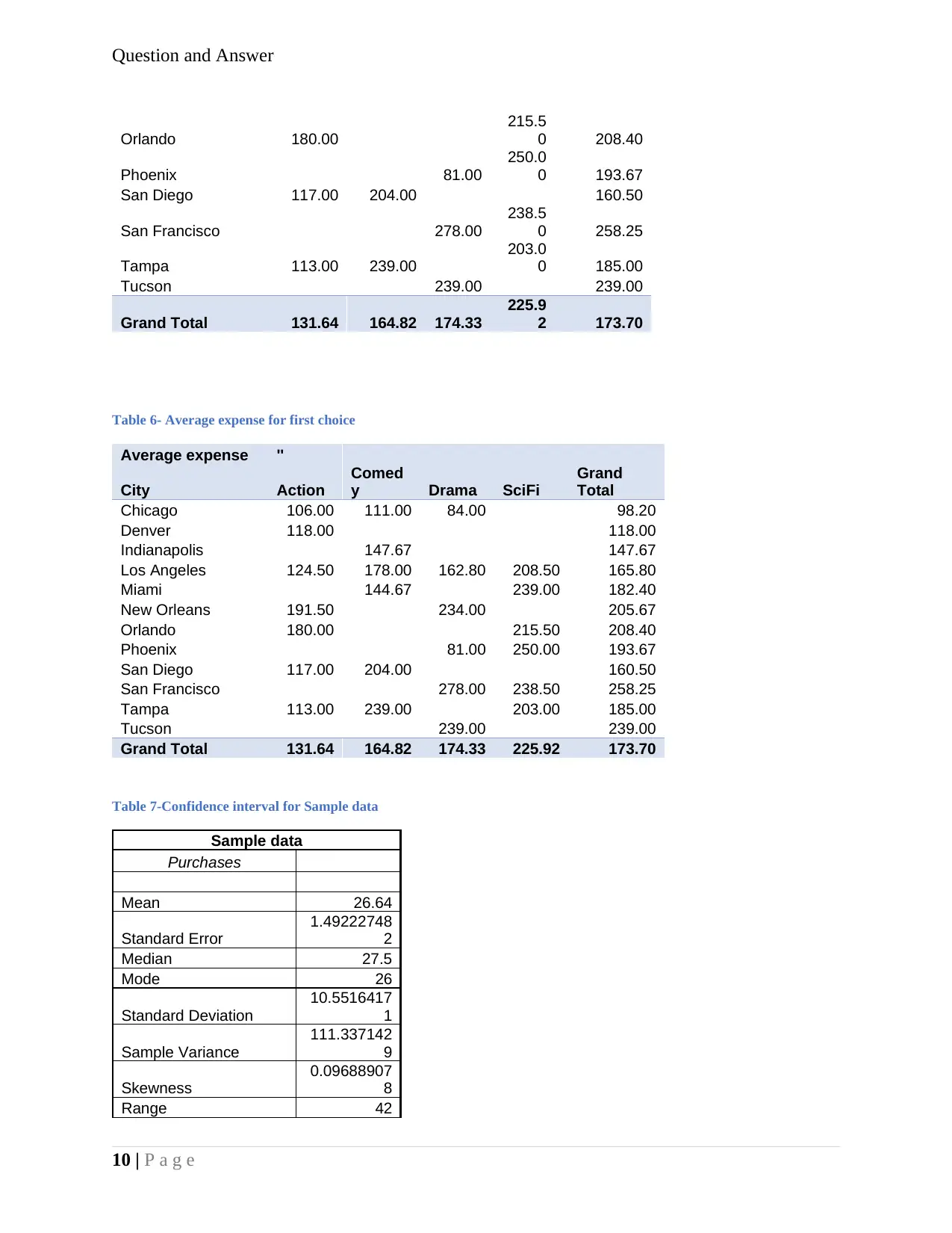
The confidence interval of four different genre of first choice is as follows
Table 5-Average number of purchases in first choice movie
Average expense ''
City
Actio
n Comedy Drama SciFi
Grand
Total
Chicago 106.00 111.00 84.00 98.20
Denver 118.00 118.00
Indianapolis 147.67 147.67
Los Angeles 124.50 178.00 162.80
208.5
0 165.80
Miami 144.67
239.0
0 182.40
New Orleans 191.50 234.00 205.67
9 | P a g e
0-14 15-24 25-34 35-44 45-54 55-64 65-74 75-84
0
500
1000
1500
2000
2500
re nc Pol on o A e an e ollarF qu y yg f g R g Vs D
Amo ntu
Figure 6 -Frequency polygon of expenditure (Age wise)
This is the frequency polygon for table 3, for which Cluster chart is also given figure 3. Almost
all the figure which is related to frequency tell only one thing that, age from 25 to 44 is the best
group for movie business purpose and this bar and frequency polygon is not different from other
frequency chart.
Solution 3
Solution 3(a)
Confidence interval – On the basis of sample data, the calculation of two numbers, which is
taken as interval, and it is supposed that, the parameter will lie within these two intervals. The
method of calculation is known s estimator and the two number are known as confidence
interval.
Suppose, a student in a practical class, calculating the boiling point of and observe the reading,
101.7, 103.5, 102.4, 100.6, 102.8, 103.5 which is six different data on samples of liquid. The
sample mean he calculated is 102.41 its deviation is 1.2 o then, its confidence interval at 95% is
1.96.
The confidence interval of four different genre of first choice is as follows
Table 5-Average number of purchases in first choice movie
Average expense ''
City
Actio
n Comedy Drama SciFi
Grand
Total
Chicago 106.00 111.00 84.00 98.20
Denver 118.00 118.00
Indianapolis 147.67 147.67
Los Angeles 124.50 178.00 162.80
208.5
0 165.80
Miami 144.67
239.0
0 182.40
New Orleans 191.50 234.00 205.67
9 | P a g e
⊘ This is a preview!⊘
Do you want full access?
Subscribe today to unlock all pages.
Trusted by 1+ million students worldwide
Question and Answer
Orlando 180.00
215.5
0 208.40
Phoenix 81.00
250.0
0 193.67
San Diego 117.00 204.00 160.50
San Francisco 278.00
238.5
0 258.25
Tampa 113.00 239.00
203.0
0 185.00
Tucson 239.00 239.00
Grand Total 131.64 164.82 174.33
225.9
2 173.70
Table 6- Average expense for first choice
Average expense ''
City Action
Comed
y Drama SciFi
Grand
Total
Chicago 106.00 111.00 84.00 98.20
Denver 118.00 118.00
Indianapolis 147.67 147.67
Los Angeles 124.50 178.00 162.80 208.50 165.80
Miami 144.67 239.00 182.40
New Orleans 191.50 234.00 205.67
Orlando 180.00 215.50 208.40
Phoenix 81.00 250.00 193.67
San Diego 117.00 204.00 160.50
San Francisco 278.00 238.50 258.25
Tampa 113.00 239.00 203.00 185.00
Tucson 239.00 239.00
Grand Total 131.64 164.82 174.33 225.92 173.70
Table 7-Confidence interval for Sample data
Sample data
Purchases
Mean 26.64
Standard Error
1.49222748
2
Median 27.5
Mode 26
Standard Deviation
10.5516417
1
Sample Variance
111.337142
9
Skewness
0.09688907
8
Range 42
10 | P a g e
Paraphrase This Document
Need a fresh take? Get an instant paraphrase of this document with our AI Paraphraser
Question and Answer
Minimum 9
Maximum 51
Sum 1332
Count 50
Confidence
Level(95.0%)
2.99874339
5
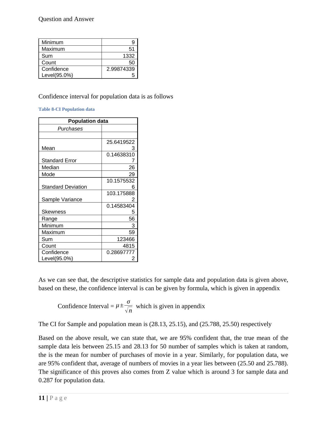
Confidence interval for population data is as follows
Table 8-CI Population data
Population data
Purchases
Mean
25.6419522
3
Standard Error
0.14638310
7
Median 26
Mode 29
Standard Deviation
10.1575532
6
Sample Variance
103.175888
2
Skewness
0.14583404
5
Range 56
Minimum 3
Maximum 59
Sum 123466
Count 4815
Confidence
Level(95.0%)
0.28697777
2
As we can see that, the descriptive statistics for sample data and population data is given above,
based on these, the confidence interval is can be given by formula, which is given in appendix
Confidence Interval = μ ± σ
√n which is given in appendix
The CI for Sample and population mean is (28.13, 25.15), and (25.788, 25.50) respectively
Based on the above result, we can state that, we are 95% confident that, the true mean of the
sample data leis between 25.15 and 28.13 for 50 number of samples which is taken at random,
the is the mean for number of purchases of movie in a year. Similarly, for population data, we
are 95% confident that, average of numbers of movies in a year lies between (25.50 and 25.788).
The significance of this proves also comes from Z value which is around 3 for sample data and
0.287 for population data.
11 | P a g e
Minimum 9
Maximum 51
Sum 1332
Count 50
Confidence
Level(95.0%)
2.99874339
5
Confidence interval for population data is as follows
Table 8-CI Population data
Population data
Purchases
Mean
25.6419522
3
Standard Error
0.14638310
7
Median 26
Mode 29
Standard Deviation
10.1575532
6
Sample Variance
103.175888
2
Skewness
0.14583404
5
Range 56
Minimum 3
Maximum 59
Sum 123466
Count 4815
Confidence
Level(95.0%)
0.28697777
2
As we can see that, the descriptive statistics for sample data and population data is given above,
based on these, the confidence interval is can be given by formula, which is given in appendix
Confidence Interval = μ ± σ
√n which is given in appendix
The CI for Sample and population mean is (28.13, 25.15), and (25.788, 25.50) respectively
Based on the above result, we can state that, we are 95% confident that, the true mean of the
sample data leis between 25.15 and 28.13 for 50 number of samples which is taken at random,
the is the mean for number of purchases of movie in a year. Similarly, for population data, we
are 95% confident that, average of numbers of movies in a year lies between (25.50 and 25.788).
The significance of this proves also comes from Z value which is around 3 for sample data and
0.287 for population data.
11 | P a g e
Question and Answer
Solution 4
Solution 4(1)
The alternative hypothesis for the given problem can be defines as
Ha :average expense offirst choice comedy> Average expense first choice drama
HO :average expense offirst choice comedy< Average expense first choice drama
After running the t-test in excel sheet, which is given in appendix, found that, the t statistics is -
0.85, t statics is less than one tail critical variable, in this condition we cannot reject null
hypothesis. Second thing is that p value is greater than α value, which also dictates that the null
hypothesis is true.
In this condition we can say that the feeling of average amount spent on comedy is more that first
choice dram movie is wrong. The average expense in first choice drama movies is more.
Solution 4(2)
The alternate hypothesis for the given test is give as
H¿ α :average purchase differ for male∧female
Ho :average purchase same for male∧female
After running the t-test for given condition, the result is obtained is given in appendix
In this result, t-stat is greater than negative of t critical two tailed test and t stat is quite
less than t critical two tailed test, in this condition, null hypothesis is rejected.
Therefore, we can say that there is difference in average purchase of male and female.
Solution 5
The regression analysis of age and dollar spent is given, after running the regression analysis, we
have achieved the figure given below.
12 | P a g e
⊘ This is a preview!⊘
Do you want full access?
Subscribe today to unlock all pages.
Trusted by 1+ million students worldwide
1 out of 22
Related Documents


Your All-in-One AI-Powered Toolkit for Academic Success.
+13062052269
info@desklib.com
Available 24*7 on WhatsApp / Email
![[object Object]](/_next/static/media/star-bottom.7253800d.svg)
Unlock your academic potential
Copyright © 2020–2026 A2Z Services. All Rights Reserved. Developed and managed by ZUCOL.