STAT6003: Financial Statistics Analysis of Market Prices

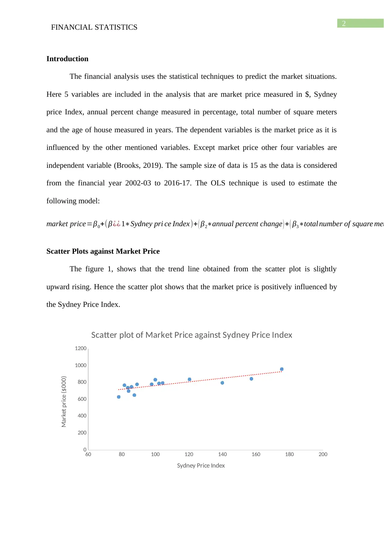
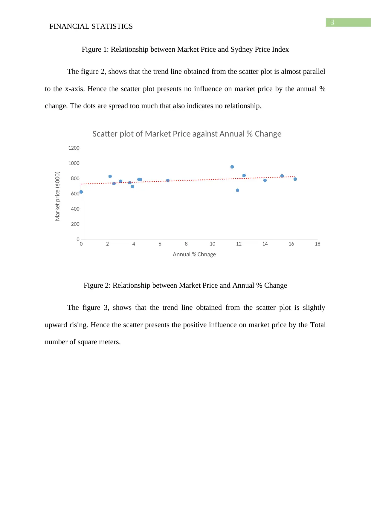
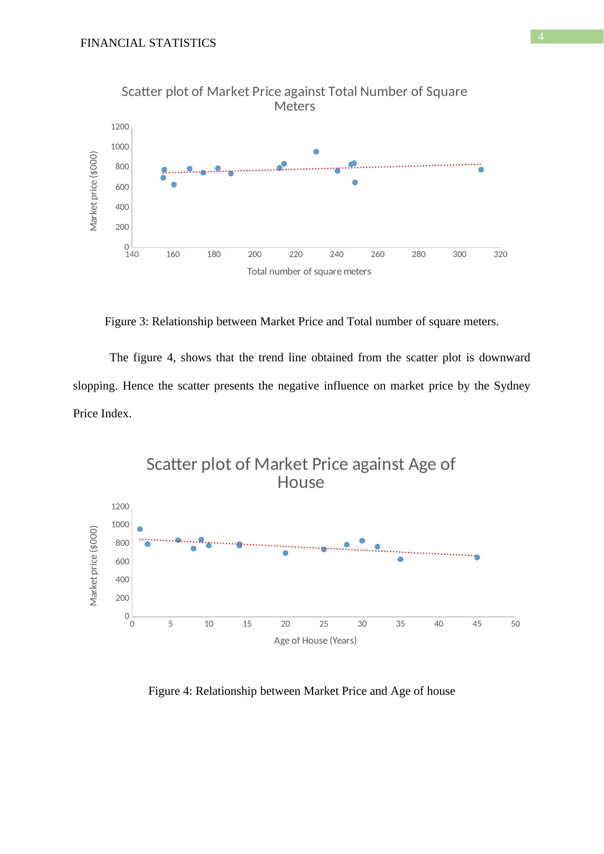
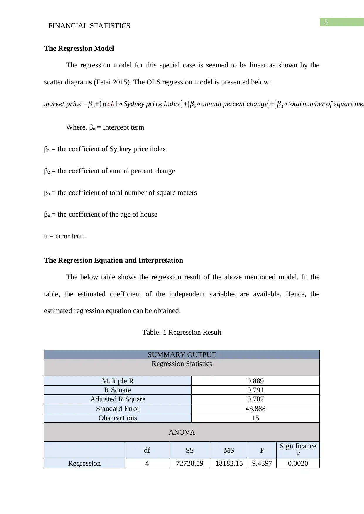
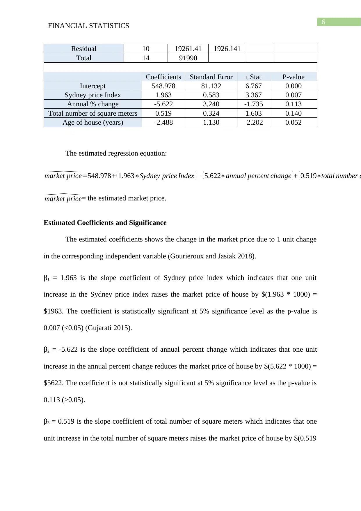
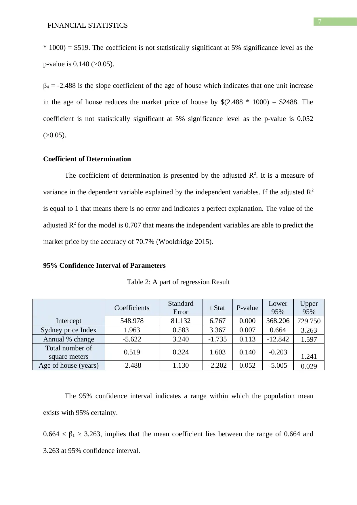
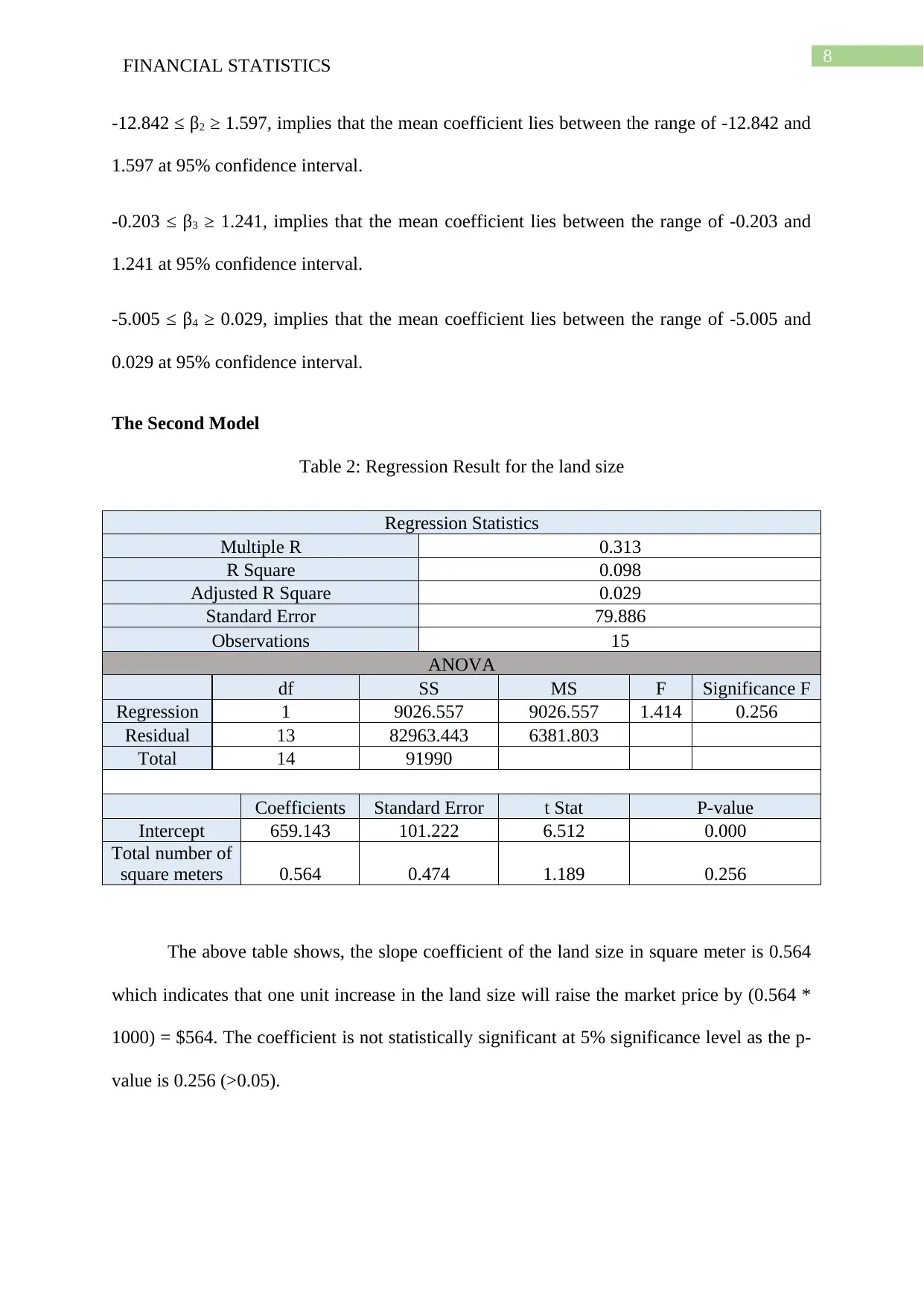
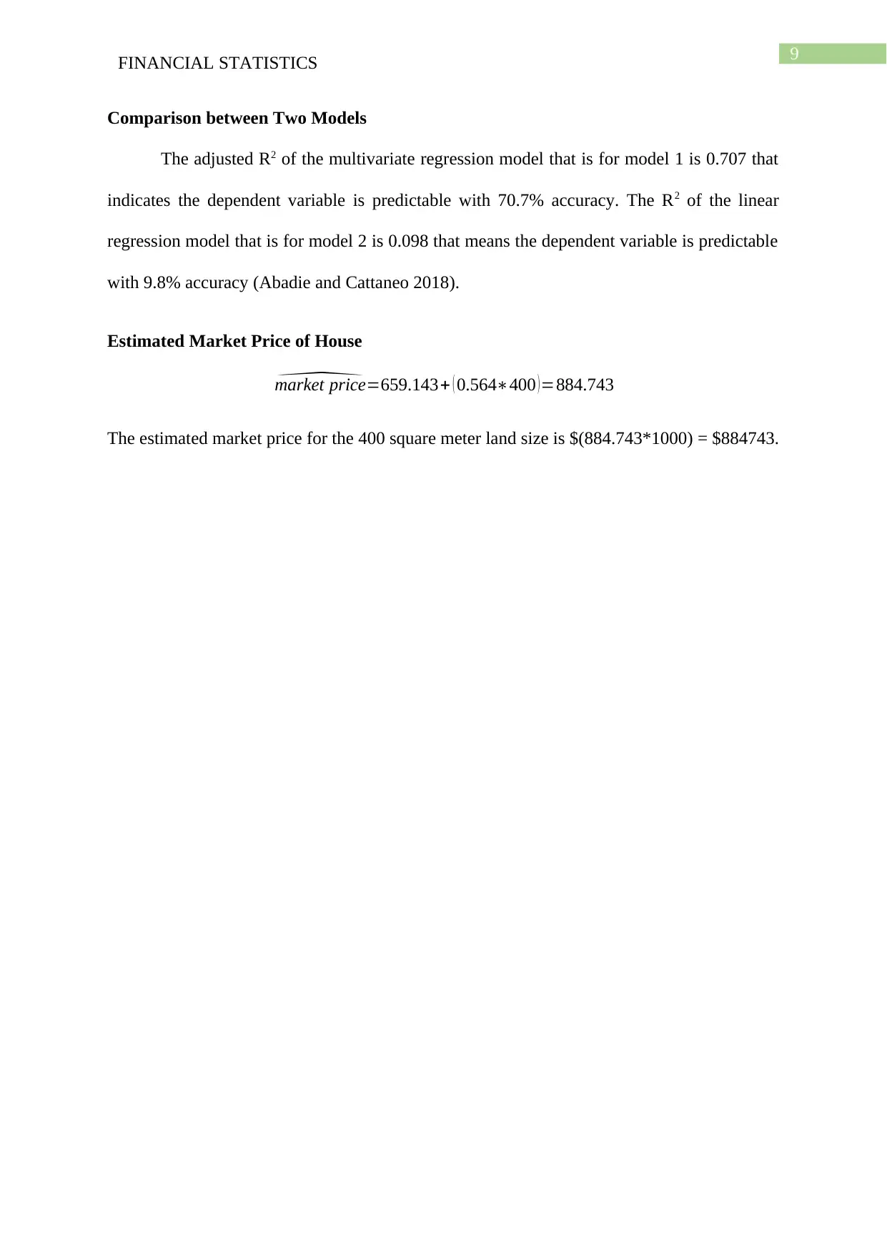
This report presents a financial statistics analysis, focusing on the relationship between market price and various economic indicators using data from 2002-2017. The analysis employs Ordinary Least Squares (OLS) regression and scatter plots to examine the influence of the Sydney Price Index, annual percentage change, total number of square meters, and age of the house on market price. The report includes the development of regression models, interpretation of coefficients, and assessment of statistical significance. The findings reveal positive correlations between market price and both the Sydney Price Index and the total number of square meters, while a negative correlation is observed with the age of the house. The report also provides a comparison between a multivariate regression model and a linear regression model, offering insights into their predictive capabilities. The report concludes with an estimated market price for a specific land size and includes relevant references.

Running head: FINANCIAL STATISTICS
Financial Statistics
Name of the Student:
Name of the University:
Author Note:

1FINANCIAL STATISTICS
Table of Contents
Introduction................................................................................................................................2
Scatter Plots against Market Price..............................................................................................2
Reference....................................................................................................................................5

2FINANCIAL STATISTICS
Introduction
The financial analysis uses the statistical techniques to predict the market situations.
Here 5 variables are included in the analysis that are market price measured in $, Sydney
price Index, annual percent change measured in percentage, total number of square meters
and the age of house measured in years. The dependent variables is the market price as it is
influenced by the other mentioned variables. Except market price other four variables are
independent variable (Brooks, 2019). The sample size of data is 15 as the data is considered
from the financial year 2002-03 to 2016-17. The OLS technique is used to estimate the
following model:
market price=β0+( β ¿¿ 1∗Sydney pri ce Index)+ ( β2∗annual percent change ) + ( β3∗total number of square met
Scatter Plots against Market Price
The figure 1, shows that the trend line obtained from the scatter plot is slightly
upward rising. Hence the scatter plot shows that the market price is positively influenced by
the Sydney Price Index.
60 80 100 120 140 160 180 200
0
200
400
600
800
1000
1200
Scatter plot of Market Price against Sydney Price Index
Sydney Price Index
Market price ($000)

3FINANCIAL STATISTICS
Figure 1: Relationship between Market Price and Sydney Price Index
The figure 2, shows that the trend line obtained from the scatter plot is almost parallel
to the x-axis. Hence the scatter plot presents no influence on market price by the annual %
change. The dots are spread too much that also indicates no relationship.
0 2 4 6 8 10 12 14 16 18
0
200
400
600
800
1000
1200
Scatter plot of Market Price against Annual % Change
Annual % Chnage
Market price ($000)
Figure 2: Relationship between Market Price and Annual % Change
The figure 3, shows that the trend line obtained from the scatter plot is slightly
upward rising. Hence the scatter presents the positive influence on market price by the Total
number of square meters.

4FINANCIAL STATISTICS
140 160 180 200 220 240 260 280 300 320
0
200
400
600
800
1000
1200
Scatter plot of Market Price against Total Number of Square
Meters
Total number of square meters
Market price ($000)
Figure 3: Relationship between Market Price and Total number of square meters.
The figure 4, shows that the trend line obtained from the scatter plot is downward
slopping. Hence the scatter presents the negative influence on market price by the Sydney
Price Index.
0 5 10 15 20 25 30 35 40 45 50
0
200
400
600
800
1000
1200
Scatter plot of Market Price against Age of
House
Age of House (Years)
Market price ($000)
Figure 4: Relationship between Market Price and Age of house

5FINANCIAL STATISTICS
The Regression Model
The regression model for this special case is seemed to be linear as shown by the
scatter diagrams (Fetai 2015). The OLS regression model is presented below:
market price=β0+( β ¿¿ 1∗Sydney pri ce Index)+ ( β2∗annual percent change ) + ( β3∗total number of square met
Where, β0 = Intercept term
β1 = the coefficient of Sydney price index
β2 = the coefficient of annual percent change
β3 = the coefficient of total number of square meters
β4 = the coefficient of the age of house
u = error term.
The Regression Equation and Interpretation
The below table shows the regression result of the above mentioned model. In the
table, the estimated coefficient of the independent variables are available. Hence, the
estimated regression equation can be obtained.
Table: 1 Regression Result
SUMMARY OUTPUT
Regression Statistics
Multiple R 0.889
R Square 0.791
Adjusted R Square 0.707
Standard Error 43.888
Observations 15
ANOVA
df SS MS F Significance
F
Regression 4 72728.59 18182.15 9.4397 0.0020

6FINANCIAL STATISTICS
Residual 10 19261.41 1926.141
Total 14 91990
Coefficients Standard Error t Stat P-value
Intercept 548.978 81.132 6.767 0.000
Sydney price Index 1.963 0.583 3.367 0.007
Annual % change -5.622 3.240 -1.735 0.113
Total number of square meters 0.519 0.324 1.603 0.140
Age of house (years) -2.488 1.130 -2.202 0.052
The estimated regression equation:
^market price=548.978+ ( 1.963∗Sydney price Index ) − ( 5.622∗annual percent change ) + ( 0.519∗total number o
^market price= the estimated market price.
Estimated Coefficients and Significance
The estimated coefficients shows the change in the market price due to 1 unit change
in the corresponding independent variable (Gourieroux and Jasiak 2018).
β1 = 1.963 is the slope coefficient of Sydney price index which indicates that one unit
increase in the Sydney price index raises the market price of house by $(1.963 * 1000) =
$1963. The coefficient is statistically significant at 5% significance level as the p-value is
0.007 (<0.05) (Gujarati 2015).
β2 = -5.622 is the slope coefficient of annual percent change which indicates that one unit
increase in the annual percent change reduces the market price of house by $(5.622 * 1000) =
$5622. The coefficient is not statistically significant at 5% significance level as the p-value is
0.113 (>0.05).
β3 = 0.519 is the slope coefficient of total number of square meters which indicates that one
unit increase in the total number of square meters raises the market price of house by $(0.519

7FINANCIAL STATISTICS
* 1000) = $519. The coefficient is not statistically significant at 5% significance level as the
p-value is 0.140 (>0.05).
β4 = -2.488 is the slope coefficient of the age of house which indicates that one unit increase
in the age of house reduces the market price of house by $(2.488 * 1000) = $2488. The
coefficient is not statistically significant at 5% significance level as the p-value is 0.052
(>0.05).
Coefficient of Determination
The coefficient of determination is presented by the adjusted R2. It is a measure of
variance in the dependent variable explained by the independent variables. If the adjusted R2
is equal to 1 that means there is no error and indicates a perfect explanation. The value of the
adjusted R2 for the model is 0.707 that means the independent variables are able to predict the
market price by the accuracy of 70.7% (Wooldridge 2015).
95% Confidence Interval of Parameters
Table 2: A part of regression Result
Coefficients Standard
Error t Stat P-value Lower
95%
Upper
95%
Intercept 548.978 81.132 6.767 0.000 368.206 729.750
Sydney price Index 1.963 0.583 3.367 0.007 0.664 3.263
Annual % change -5.622 3.240 -1.735 0.113 -12.842 1.597
Total number of
square meters 0.519 0.324 1.603 0.140 -0.203 1.241
Age of house (years) -2.488 1.130 -2.202 0.052 -5.005 0.029
The 95% confidence interval indicates a range within which the population mean
exists with 95% certainty.
0.664 ≤ β1 ≥ 3.263, implies that the mean coefficient lies between the range of 0.664 and
3.263 at 95% confidence interval.

8FINANCIAL STATISTICS
-12.842 ≤ β2 ≥ 1.597, implies that the mean coefficient lies between the range of -12.842 and
1.597 at 95% confidence interval.
-0.203 ≤ β3 ≥ 1.241, implies that the mean coefficient lies between the range of -0.203 and
1.241 at 95% confidence interval.
-5.005 ≤ β4 ≥ 0.029, implies that the mean coefficient lies between the range of -5.005 and
0.029 at 95% confidence interval.
The Second Model
Table 2: Regression Result for the land size
Regression Statistics
Multiple R 0.313
R Square 0.098
Adjusted R Square 0.029
Standard Error 79.886
Observations 15
ANOVA
df SS MS F Significance F
Regression 1 9026.557 9026.557 1.414 0.256
Residual 13 82963.443 6381.803
Total 14 91990
Coefficients Standard Error t Stat P-value
Intercept 659.143 101.222 6.512 0.000
Total number of
square meters 0.564 0.474 1.189 0.256
The above table shows, the slope coefficient of the land size in square meter is 0.564
which indicates that one unit increase in the land size will raise the market price by (0.564 *
1000) = $564. The coefficient is not statistically significant at 5% significance level as the p-
value is 0.256 (>0.05).

9FINANCIAL STATISTICS
Comparison between Two Models
The adjusted R2 of the multivariate regression model that is for model 1 is 0.707 that
indicates the dependent variable is predictable with 70.7% accuracy. The R2 of the linear
regression model that is for model 2 is 0.098 that means the dependent variable is predictable
with 9.8% accuracy (Abadie and Cattaneo 2018).
Estimated Market Price of House
^market price=659.143+ ( 0.564∗400 )=884.743
The estimated market price for the 400 square meter land size is $(884.743*1000) = $884743.

10FINANCIAL STATISTICS
Reference
Abadie, A. and Cattaneo, M.D., 2018. Econometric methods for program evaluation. Annual
Review of Economics, 10, pp.465-503.
Brooks, C., 2019. Introductory econometrics for finance. Cambridge university press.
Fetai, B., 2015. Financial integration and financial development: does financial integration
metter?. European Research Studies, 18(2), p.97.
Gourieroux, C. and Jasiak, J., 2018. Financial econometrics: Problems, models, and methods.
PrinceFan, J. and Yao, Q., 2017. The elements of financial econometrics. Cambridge
University Press.ton University Press.
Gujarati, D., 2015. Econometrics (by example second edition). China: Palgrave.
Vogel, H.L., 2018. Financial Market Bubbles and Crashes: Features, Causes, and Effects.
Springer.
Wooldridge, J.M., 2015. Introductory econometrics: A modern approach. Nelson Education.