Econometrics Analysis of Financial Time Series Assignment

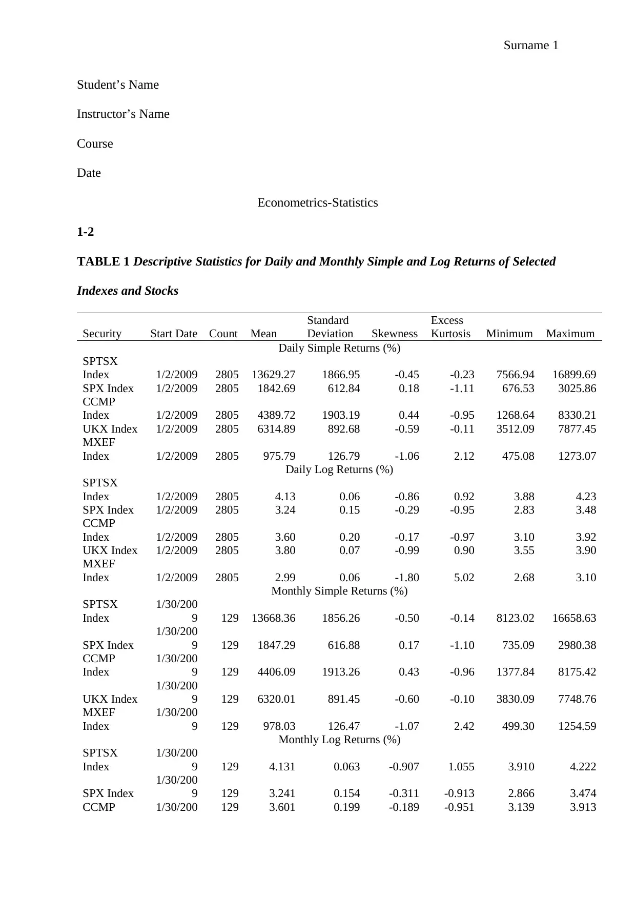
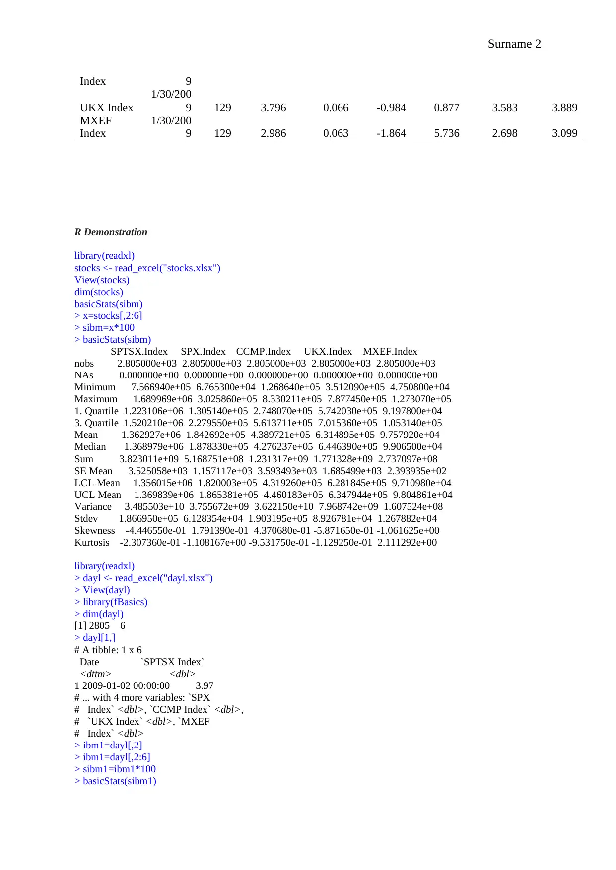
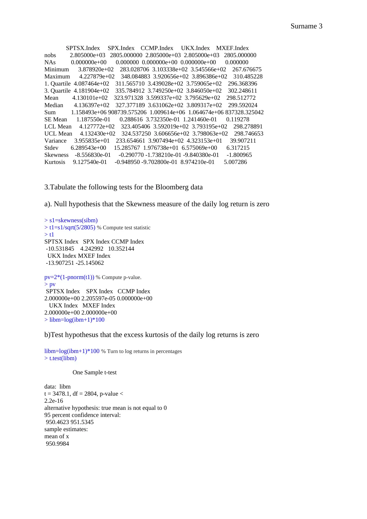
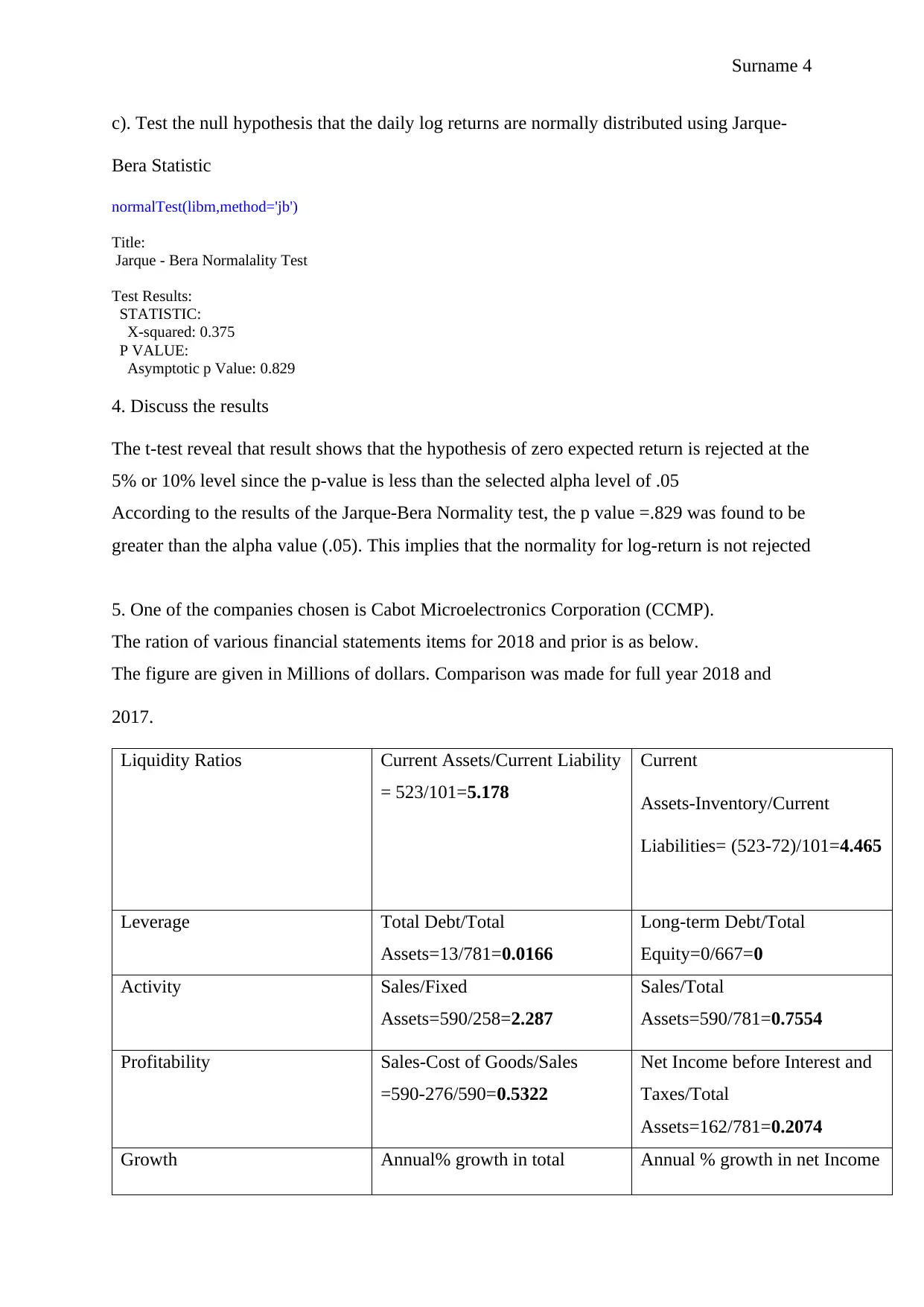
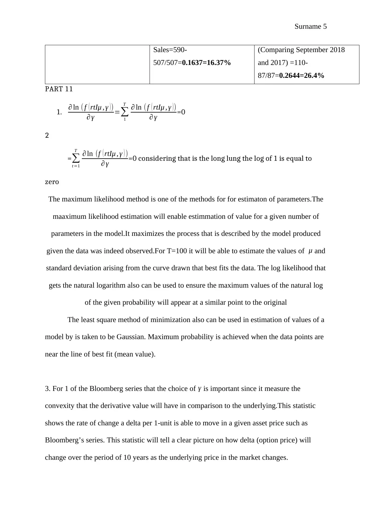
This assignment analyzes financial time series data using econometrics and R programming. It begins with descriptive statistics of daily and monthly simple and log returns for various indexes and stocks, including SPTSX, SPX, CCMP, UKX, and MXEF. The analysis involves calculating mean, standard deviation, skewness, and kurtosis. The assignment then uses R code to import data and calculate basic statistics using the 'fBasics' package. Further, the assignment involves performing hypothesis tests for skewness and excess kurtosis of daily log returns, including the computation of test statistics and p-values. The Jarque-Bera test is applied to assess the normality of the returns. The assignment includes a financial statement analysis of Cabot Microelectronics Corporation (CCMP), calculating liquidity, leverage, activity, profitability, and growth ratios for 2018 and 2017. Finally, it discusses concepts such as maximum likelihood estimation, the importance of delta in financial series, and whether the likelihood function can be considered a joint probability density function.

Surname 1
Student’s Name
Instructor’s Name
Course
Date
Econometrics-Statistics
1-2
TABLE 1 Descriptive Statistics for Daily and Monthly Simple and Log Returns of Selected
Indexes and Stocks
Security Start Date Count Mean
Standard
Deviation Skewness
Excess
Kurtosis Minimum Maximum
Daily Simple Returns (%)
SPTSX
Index 1/2/2009 2805 13629.27 1866.95 -0.45 -0.23 7566.94 16899.69
SPX Index 1/2/2009 2805 1842.69 612.84 0.18 -1.11 676.53 3025.86
CCMP
Index 1/2/2009 2805 4389.72 1903.19 0.44 -0.95 1268.64 8330.21
UKX Index 1/2/2009 2805 6314.89 892.68 -0.59 -0.11 3512.09 7877.45
MXEF
Index 1/2/2009 2805 975.79 126.79 -1.06 2.12 475.08 1273.07
Daily Log Returns (%)
SPTSX
Index 1/2/2009 2805 4.13 0.06 -0.86 0.92 3.88 4.23
SPX Index 1/2/2009 2805 3.24 0.15 -0.29 -0.95 2.83 3.48
CCMP
Index 1/2/2009 2805 3.60 0.20 -0.17 -0.97 3.10 3.92
UKX Index 1/2/2009 2805 3.80 0.07 -0.99 0.90 3.55 3.90
MXEF
Index 1/2/2009 2805 2.99 0.06 -1.80 5.02 2.68 3.10
Monthly Simple Returns (%)
SPTSX
Index
1/30/200
9 129 13668.36 1856.26 -0.50 -0.14 8123.02 16658.63
SPX Index
1/30/200
9 129 1847.29 616.88 0.17 -1.10 735.09 2980.38
CCMP
Index
1/30/200
9 129 4406.09 1913.26 0.43 -0.96 1377.84 8175.42
UKX Index
1/30/200
9 129 6320.01 891.45 -0.60 -0.10 3830.09 7748.76
MXEF
Index
1/30/200
9 129 978.03 126.47 -1.07 2.42 499.30 1254.59
Monthly Log Returns (%)
SPTSX
Index
1/30/200
9 129 4.131 0.063 -0.907 1.055 3.910 4.222
SPX Index
1/30/200
9 129 3.241 0.154 -0.311 -0.913 2.866 3.474
CCMP 1/30/200 129 3.601 0.199 -0.189 -0.951 3.139 3.913

Surname 2
Index 9
UKX Index
1/30/200
9 129 3.796 0.066 -0.984 0.877 3.583 3.889
MXEF
Index
1/30/200
9 129 2.986 0.063 -1.864 5.736 2.698 3.099
R Demonstration
library(readxl)
stocks <- read_excel("stocks.xlsx")
View(stocks)
dim(stocks)
basicStats(sibm)
> x=stocks[,2:6]
> sibm=x*100
> basicStats(sibm)
SPTSX.Index SPX.Index CCMP.Index UKX.Index MXEF.Index
nobs 2.805000e+03 2.805000e+03 2.805000e+03 2.805000e+03 2.805000e+03
NAs 0.000000e+00 0.000000e+00 0.000000e+00 0.000000e+00 0.000000e+00
Minimum 7.566940e+05 6.765300e+04 1.268640e+05 3.512090e+05 4.750800e+04
Maximum 1.689969e+06 3.025860e+05 8.330211e+05 7.877450e+05 1.273070e+05
1. Quartile 1.223106e+06 1.305140e+05 2.748070e+05 5.742030e+05 9.197800e+04
3. Quartile 1.520210e+06 2.279550e+05 5.613711e+05 7.015360e+05 1.053140e+05
Mean 1.362927e+06 1.842692e+05 4.389721e+05 6.314895e+05 9.757920e+04
Median 1.368979e+06 1.878330e+05 4.276237e+05 6.446390e+05 9.906500e+04
Sum 3.823011e+09 5.168751e+08 1.231317e+09 1.771328e+09 2.737097e+08
SE Mean 3.525058e+03 1.157117e+03 3.593493e+03 1.685499e+03 2.393935e+02
LCL Mean 1.356015e+06 1.820003e+05 4.319260e+05 6.281845e+05 9.710980e+04
UCL Mean 1.369839e+06 1.865381e+05 4.460183e+05 6.347944e+05 9.804861e+04
Variance 3.485503e+10 3.755672e+09 3.622150e+10 7.968742e+09 1.607524e+08
Stdev 1.866950e+05 6.128354e+04 1.903195e+05 8.926781e+04 1.267882e+04
Skewness -4.446550e-01 1.791390e-01 4.370680e-01 -5.871650e-01 -1.061625e+00
Kurtosis -2.307360e-01 -1.108167e+00 -9.531750e-01 -1.129250e-01 2.111292e+00
library(readxl)
> dayl <- read_excel("dayl.xlsx")
> View(dayl)
> library(fBasics)
> dim(dayl)
[1] 2805 6
> dayl[1,]
# A tibble: 1 x 6
Date `SPTSX Index`
<dttm> <dbl>
1 2009-01-02 00:00:00 3.97
# ... with 4 more variables: `SPX
# Index` <dbl>, `CCMP Index` <dbl>,
# `UKX Index` <dbl>, `MXEF
# Index` <dbl>
> ibm1=dayl[,2]
> ibm1=dayl[,2:6]
> sibm1=ibm1*100
> basicStats(sibm1)

Surname 3
SPTSX.Index SPX.Index CCMP.Index UKX.Index MXEF.Index
nobs 2.805000e+03 2805.000000 2.805000e+03 2.805000e+03 2805.000000
NAs 0.000000e+00 0.000000 0.000000e+00 0.000000e+00 0.000000
Minimum 3.878920e+02 283.028706 3.103338e+02 3.545566e+02 267.676675
Maximum 4.227879e+02 348.084883 3.920656e+02 3.896386e+02 310.485228
1. Quartile 4.087464e+02 311.565710 3.439028e+02 3.759065e+02 296.368396
3. Quartile 4.181904e+02 335.784912 3.749250e+02 3.846050e+02 302.248611
Mean 4.130101e+02 323.971328 3.599337e+02 3.795629e+02 298.512772
Median 4.136397e+02 327.377189 3.631062e+02 3.809317e+02 299.592024
Sum 1.158493e+06 908739.575206 1.009614e+06 1.064674e+06 837328.325042
SE Mean 1.187550e-01 0.288616 3.732350e-01 1.241460e-01 0.119278
LCL Mean 4.127772e+02 323.405406 3.592019e+02 3.793195e+02 298.278891
UCL Mean 4.132430e+02 324.537250 3.606656e+02 3.798063e+02 298.746653
Variance 3.955835e+01 233.654661 3.907494e+02 4.323153e+01 39.907211
Stdev 6.289543e+00 15.285767 1.976738e+01 6.575069e+00 6.317215
Skewness -8.556830e-01 -0.290770 -1.738210e-01 -9.840380e-01 -1.800965
Kurtosis 9.127540e-01 -0.948950 -9.702800e-01 8.974210e-01 5.007286
3.Tabulate the following tests for the Bloomberg data
a). Null hypothesis that the Skewness measure of the daily log return is zero
> s1=skewness(sibm)
> t1=s1/sqrt(5/2805) % Compute test statistic
> t1
SPTSX Index SPX Index CCMP Index
-10.531845 4.242992 10.352144
UKX Index MXEF Index
-13.907251 -25.145062
pv=2*(1-pnorm(t1)) % Compute p-value.
> pv
SPTSX Index SPX Index CCMP Index
2.000000e+00 2.205597e-05 0.000000e+00
UKX Index MXEF Index
2.000000e+00 2.000000e+00
> libm=log(ibm+1)*100
b)Test hypothesus that the excess kurtosis of the daily log returns is zero
libm=log(ibm+1)*100 % Turn to log returns in percentages
> t.test(libm)
One Sample t-test
data: libm
t = 3478.1, df = 2804, p-value <
2.2e-16
alternative hypothesis: true mean is not equal to 0
95 percent confidence interval:
950.4623 951.5345
sample estimates:
mean of x
950.9984

Surname 4
c). Test the null hypothesis that the daily log returns are normally distributed using Jarque-
Bera Statistic
normalTest(libm,method='jb')
Title:
Jarque - Bera Normalality Test
Test Results:
STATISTIC:
X-squared: 0.375
P VALUE:
Asymptotic p Value: 0.829
4. Discuss the results
The t-test reveal that result shows that the hypothesis of zero expected return is rejected at the
5% or 10% level since the p-value is less than the selected alpha level of .05
According to the results of the Jarque-Bera Normality test, the p value =.829 was found to be
greater than the alpha value (.05). This implies that the normality for log-return is not rejected
5. One of the companies chosen is Cabot Microelectronics Corporation (CCMP).
The ration of various financial statements items for 2018 and prior is as below.
The figure are given in Millions of dollars. Comparison was made for full year 2018 and
2017.
Liquidity Ratios Current Assets/Current Liability
= 523/101=5.178
Current
Assets-Inventory/Current
Liabilities= (523-72)/101=4.465
Leverage Total Debt/Total
Assets=13/781=0.0166
Long-term Debt/Total
Equity=0/667=0
Activity Sales/Fixed
Assets=590/258=2.287
Sales/Total
Assets=590/781=0.7554
Profitability Sales-Cost of Goods/Sales
=590-276/590=0.5322
Net Income before Interest and
Taxes/Total
Assets=162/781=0.2074
Growth Annual% growth in total Annual % growth in net Income

Surname 5
Sales=590-
507/507=0.1637=16.37%
(Comparing September 2018
and 2017) =110-
87/87=0.2644=26.4%
PART 11
1. ∂ ln ( f ( rtIμ , γ ))
∂ γ =∑
1
T ∂ ln (f ( rtIμ , γ ))
∂ γ =0
2
=∑
t =1
T ∂ ln (f ( rtIμ , γ ) )
∂ γ =0 considering that is the long lung the log of 1 is equal to
zero
The maximum likelihood method is one of the methods for for estimaton of parameters.The
maaximum likelihood estimation will enable estimmation of value for a given number of
parameters in the model.It maximizes the process that is described by the model produced
given the data was indeed observed.For T=100 it will be able to estimate the values of μ and
standard deviation arising from the curve drawn that best fits the data. The log likelihood that
gets the natural logarithm also can be used to ensure the maximum values of the natural log
of the given probability will appear at a similar point to the original
The least square method of minimization also can be used in estimation of values of a
model by is taken to be Gaussian. Maximum probability is achieved when the data points are
near the line of best fit (mean value).
3. For 1 of the Bloomberg series that the choice of γ is important since it measure the
convexity that the derivative value will have in comparison to the underlying.This statistic
shows the rate of change a delta per 1-unit is able to move in a given asset price such as
Bloomberg’s series. This statistic will tell a clear picture on how delta (option price) will
change over the period of 10 years as the underlying price in the market changes.

Surname 6
4. Likelihood be considered a joint pdf? Explain why or why not
A probability density function is taken as non-negative function that integrates to
1.Notably, the likelihood function is usually a function derived from an unknown parameter
give asθ.This is usually conditioned on the data given. It is therefore does not typically
represent an area of 1 as it is normally suggested. The integral of the function over all
possible value that θ can acquire does not equal 1.This therefore makes its not to satisfy the
definition of a pdf.
On the other hand, likelihood function can be said to be a joint probability density for an
observed data provided with the parameter θ.This function can be easily normalized to result
to a density function. This therefore suggests its likelihood to be a probability distribution
function.