Financial Econometrics Report: Time Series Analysis and Forecasting

This report delves into financial econometrics, applying statistical methods to financial market data. It identifies and estimates time series models, evaluates sub-sample forecasts, and analyzes the characteristics of returns. The report examines the impact of oil price shocks on financial variables, including market volatility and equity returns, along with the influence of Economic Policy Uncertainty (EPU) on bond spreads and volatility. Furthermore, it tests hypotheses concerning private consumption expenditure, its relationship with financial wealth and labor income, and its predictive power for future consumption and equity returns. The analysis employs VAR models and Granger causality tests to establish relationships between variables and assess the effects of shocks. The report provides a comprehensive analysis of financial market dynamics.

FINANCIAL
ECONOMETRICS

TABLE OF CONTENTS
INTRODUCTION...........................................................................................................................1
QUESTION 1...................................................................................................................................1
(a) Identifying and estimating time series model........................................................................1
(b) Using sub sample obtained in and out of sample forecasts and evaluating chosen models..4
QUESTION 3...................................................................................................................................7
(a) Calculating effect of shocks of oil prices on financial variables...........................................7
(b) Establishing that development in equity market impact volatility......................................12
(c) Impact of EPU on bond spread and volatility index............................................................13
QUESTION 4.................................................................................................................................16
(a) Testing the hypothesis that private consumption expenditure is related to financial wealth
and labour income.....................................................................................................................16
(b) Forecasting future private consumption expenditure.........................................................18
(c) Testing the hypothesis that ‘excess’ private consumption expenditure is a useful predictor
of excess equity returns.............................................................................................................20
CONCLUSION..............................................................................................................................21
REFERENCES..............................................................................................................................22

INTRODUCTION
Financial econometrics is known as application of statistical method to data of financial
market. It is considered as branch of financial economics and helps in studying quantitative
problems arise through management. The present report would identify and estimate time series
model and sub sample obtained in and out of forecasts of sample. It will consider series of
returns and examined about normality with important characteristic of distributions of returns. In
the same series, it will estimate model of conditional variance and motivation with use along
with incorporation of specification both sign and relative size of shock with impact in condition
volatility (Li and et.al., 2019). Moreover, it will extract impact of shocks to prices of oil on
particular financial variables and development in equity markets which impact volatility.
Simultaneously, it will show impact of EPU on spread of bond and affected through volatility
index. This report will test hypothesis that private consumption expenditure is related to two of
sources and way to predict future private consumption expenditure. Lastly, hypothesis would be
testes about excess private consumption expenditure as useful predictor of excess returns of
equity.
QUESTION 1
(a) Identifying and estimating time series model
On basis of identifying and determining time series model, there is evaluation of the least
square model which is form of mathematical regression that extracts line of best fit for particular
set of data, giving visual demonstration of relationship among different data points. Every point
of data is replicated as representative of relationship within independent variable and unknown
dependent variable. It gives overall rationale for placement of the line of appropriate fit within
data points being elaborated (Nguyen, 2019). The very common application of method of the
least squares which is replicated as linear or ordinary with objective of creating a straight line
that reduces sum of squares of errors produced by outcomes of associated equations like
associated equations like squared residuals from variations in observed value and anticipated on
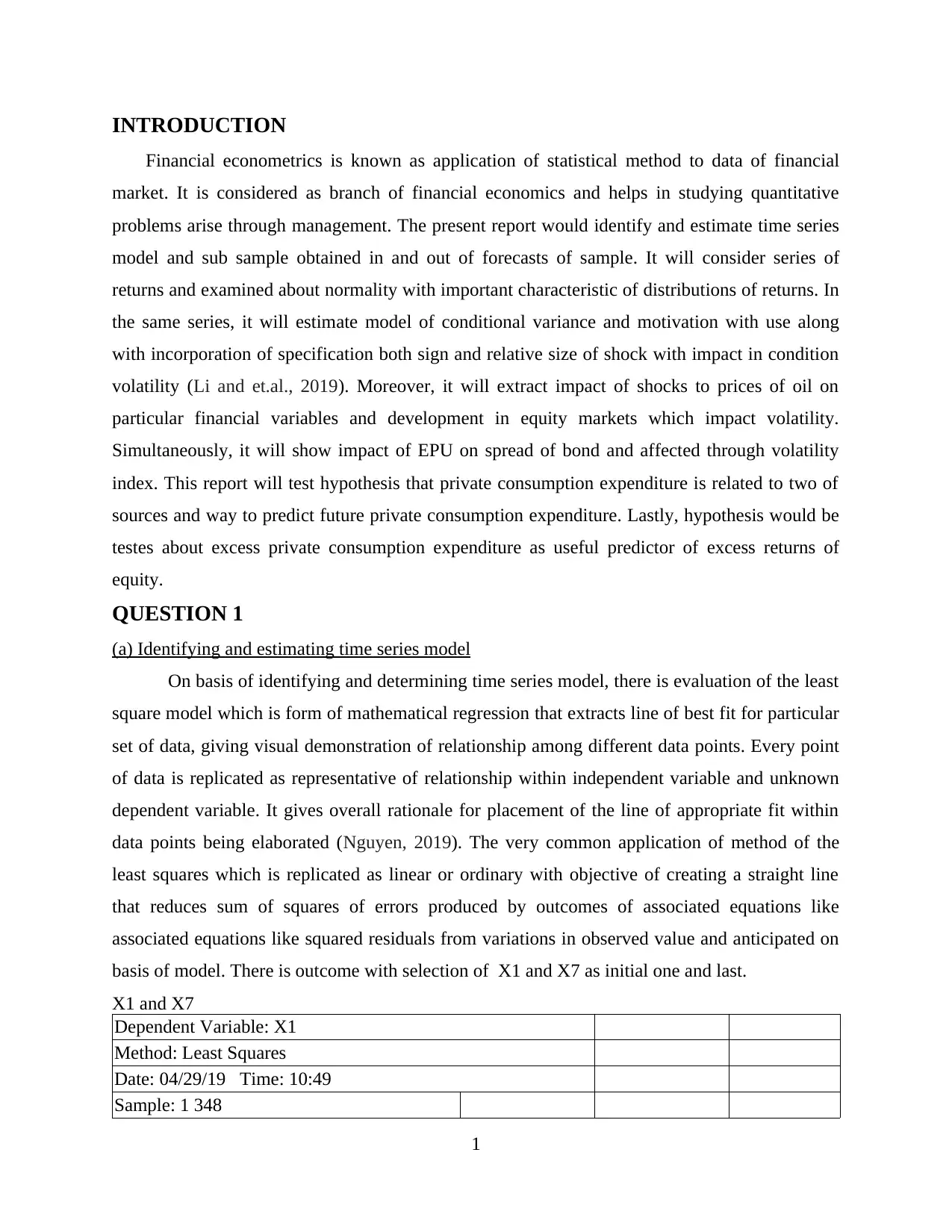
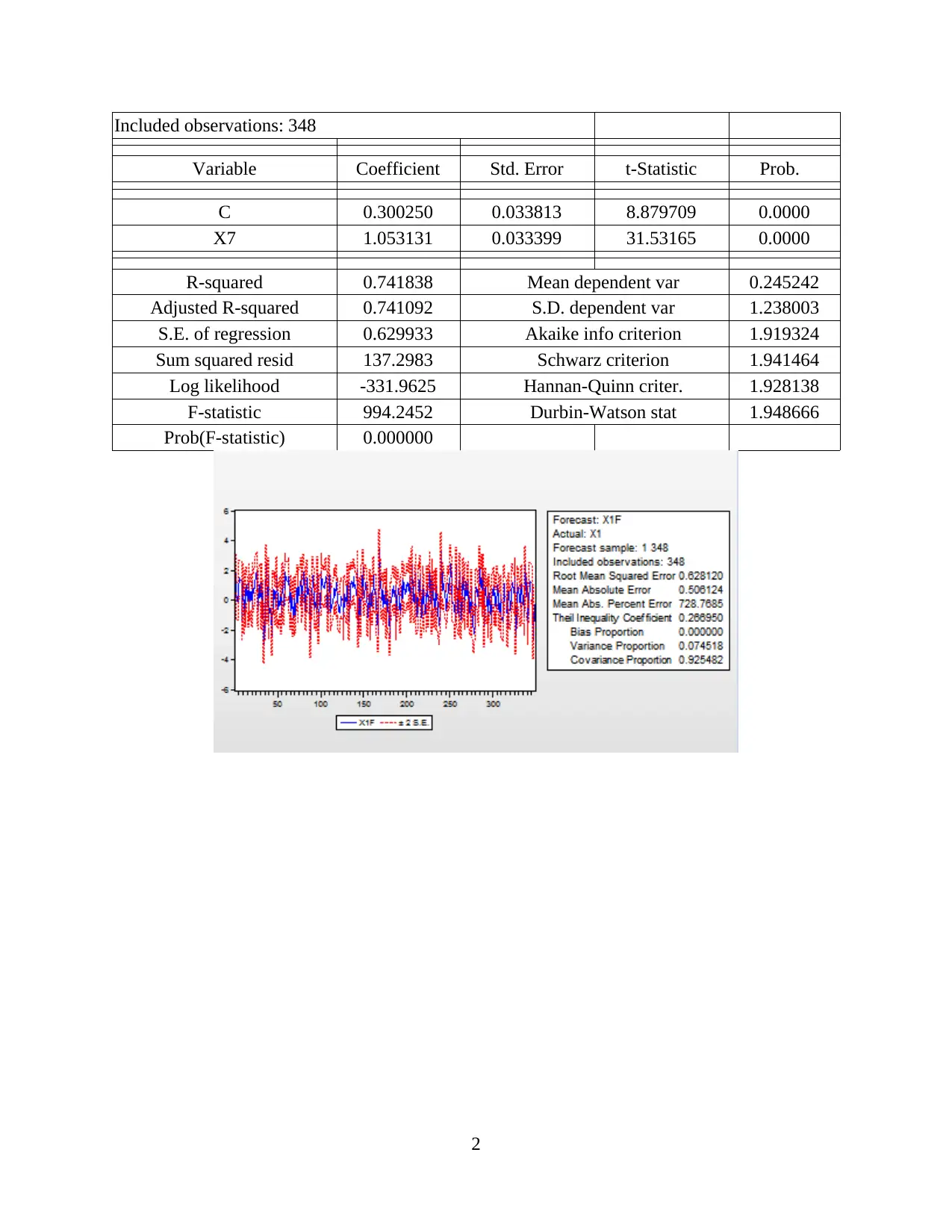
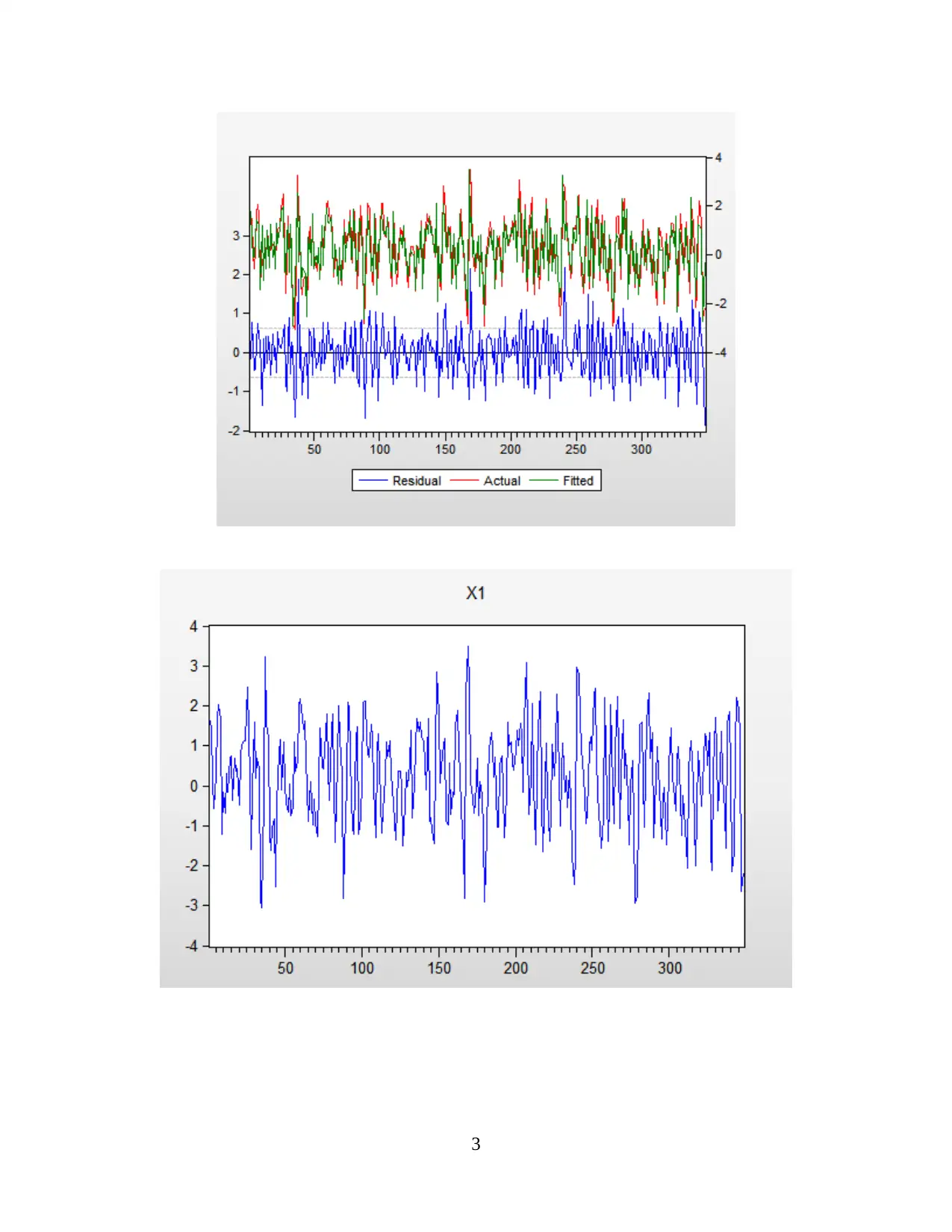
basis of model. There is outcome with selection of X1 and X7 as initial one and last.
X1 and X7
Dependent Variable: X1
Method: Least Squares
Date: 04/29/19 Time: 10:49
Sample: 1 348
1

Included observations: 348
Variable Coefficient Std. Error t-Statistic Prob.
C 0.300250 0.033813 8.879709 0.0000
X7 1.053131 0.033399 31.53165 0.0000
R-squared 0.741838 Mean dependent var 0.245242
Adjusted R-squared 0.741092 S.D. dependent var 1.238003
S.E. of regression 0.629933 Akaike info criterion 1.919324
Sum squared resid 137.2983 Schwarz criterion 1.941464
Log likelihood -331.9625 Hannan-Quinn criter. 1.928138
F-statistic 994.2452 Durbin-Watson stat 1.948666
Prob(F-statistic) 0.000000
2

3

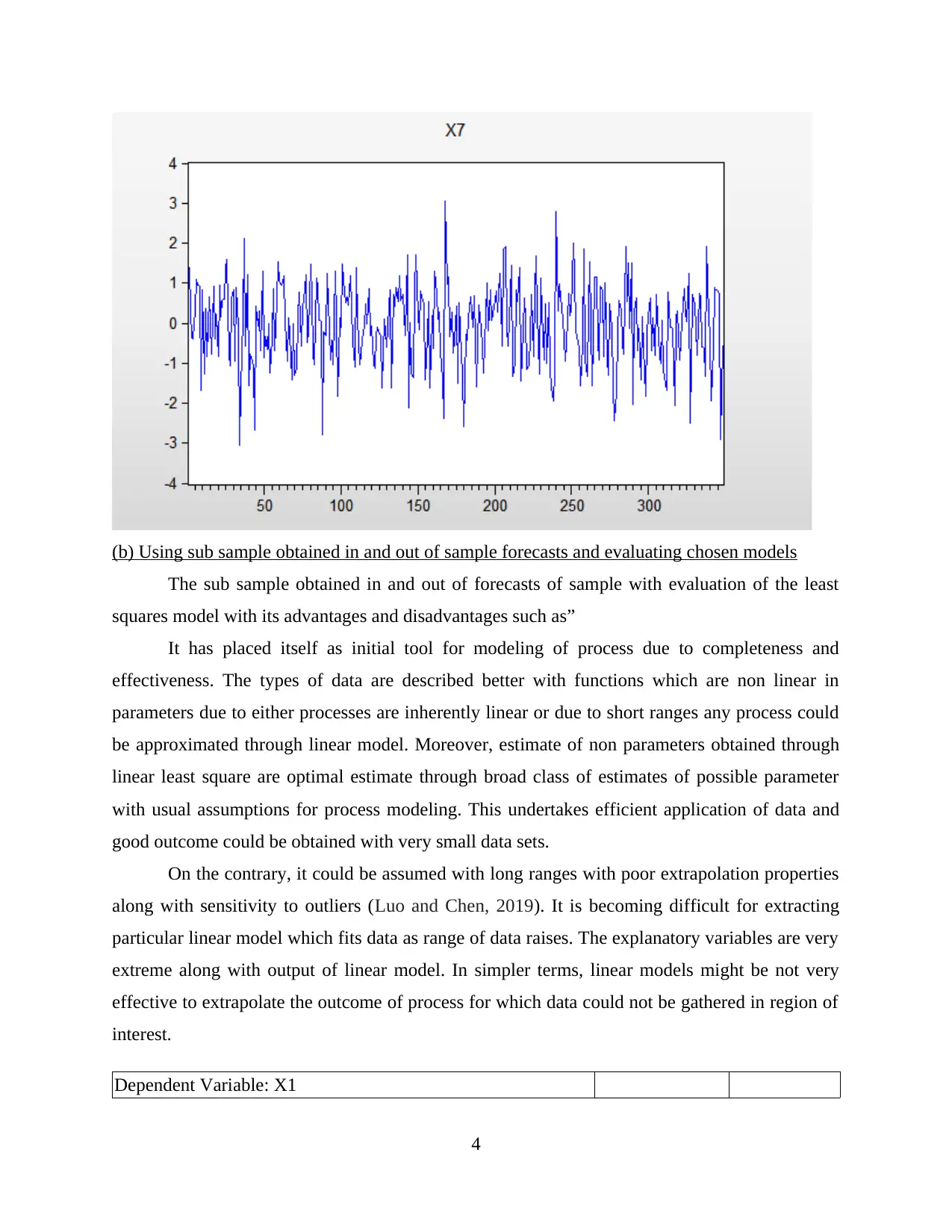
(b) Using sub sample obtained in and out of sample forecasts and evaluating chosen models
The sub sample obtained in and out of forecasts of sample with evaluation of the least
squares model with its advantages and disadvantages such as”
It has placed itself as initial tool for modeling of process due to completeness and
effectiveness. The types of data are described better with functions which are non linear in
parameters due to either processes are inherently linear or due to short ranges any process could
be approximated through linear model. Moreover, estimate of non parameters obtained through
linear least square are optimal estimate through broad class of estimates of possible parameter
with usual assumptions for process modeling. This undertakes efficient application of data and
good outcome could be obtained with very small data sets.
On the contrary, it could be assumed with long ranges with poor extrapolation properties
along with sensitivity to outliers (Luo and Chen, 2019). It is becoming difficult for extracting
particular linear model which fits data as range of data raises. The explanatory variables are very
extreme along with output of linear model. In simpler terms, linear models might be not very
effective to extrapolate the outcome of process for which data could not be gathered in region of
interest.
Dependent Variable: X1
4

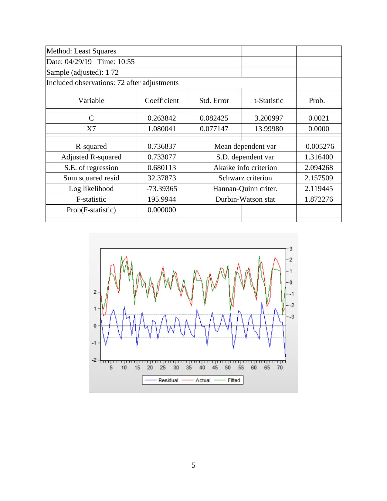
Method: Least Squares
Date: 04/29/19 Time: 10:55
Sample (adjusted): 1 72
Included observations: 72 after adjustments
Variable Coefficient Std. Error t-Statistic Prob.
C 0.263842 0.082425 3.200997 0.0021
X7 1.080041 0.077147 13.99980 0.0000
R-squared 0.736837 Mean dependent var -0.005276
Adjusted R-squared 0.733077 S.D. dependent var 1.316400
S.E. of regression 0.680113 Akaike info criterion 2.094268
Sum squared resid 32.37873 Schwarz criterion 2.157509
Log likelihood -73.39365 Hannan-Quinn criter. 2.119445
F-statistic 195.9944 Durbin-Watson stat 1.872276
Prob(F-statistic) 0.000000
5

6

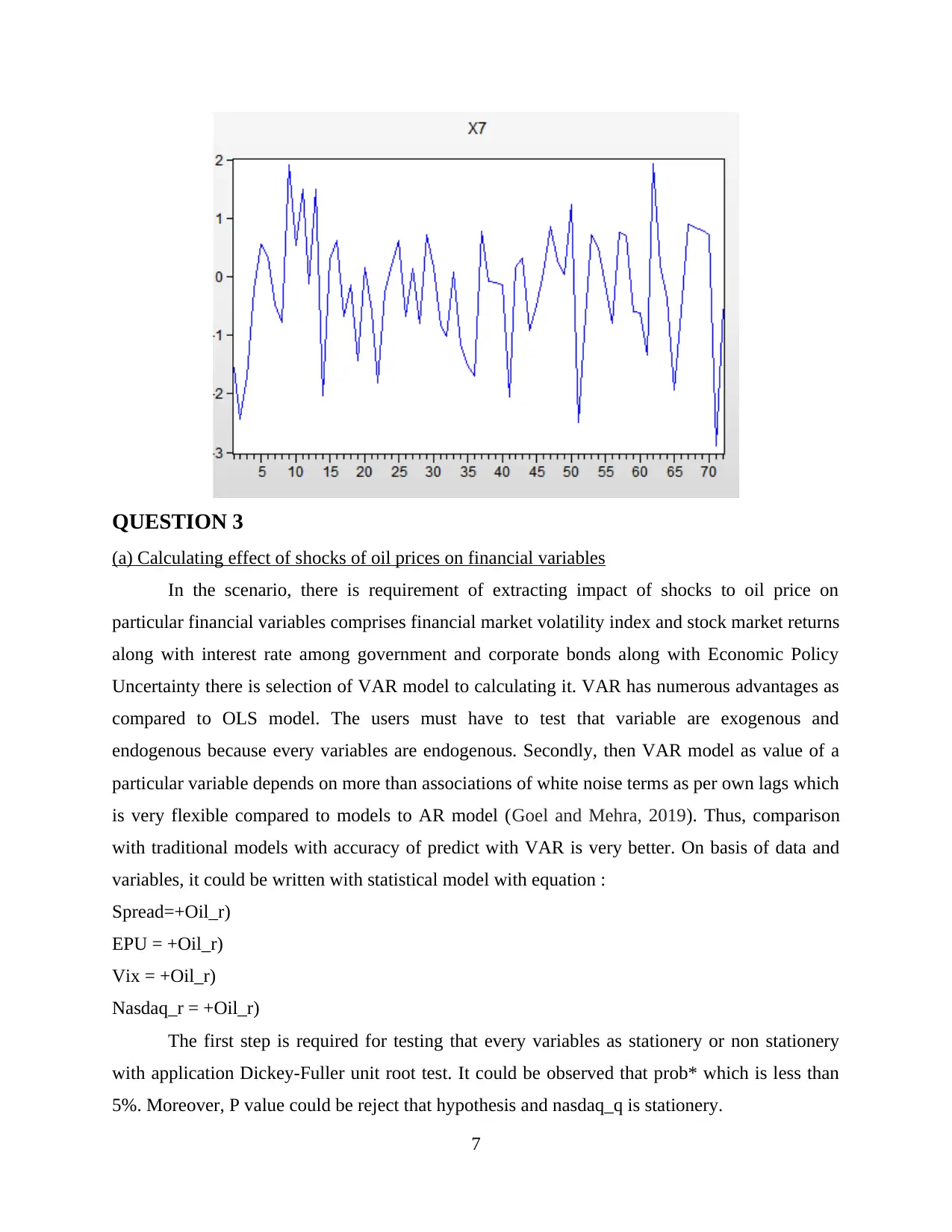
QUESTION 3
(a) Calculating effect of shocks of oil prices on financial variables
In the scenario, there is requirement of extracting impact of shocks to oil price on
particular financial variables comprises financial market volatility index and stock market returns
along with interest rate among government and corporate bonds along with Economic Policy
Uncertainty there is selection of VAR model to calculating it. VAR has numerous advantages as
compared to OLS model. The users must have to test that variable are exogenous and
endogenous because every variables are endogenous. Secondly, then VAR model as value of a
particular variable depends on more than associations of white noise terms as per own lags which
is very flexible compared to models to AR model (Goel and Mehra, 2019). Thus, comparison
with traditional models with accuracy of predict with VAR is very better. On basis of data and
variables, it could be written with statistical model with equation :
Spread=+Oil_r)
EPU = +Oil_r)
Vix = +Oil_r)
Nasdaq_r = +Oil_r)
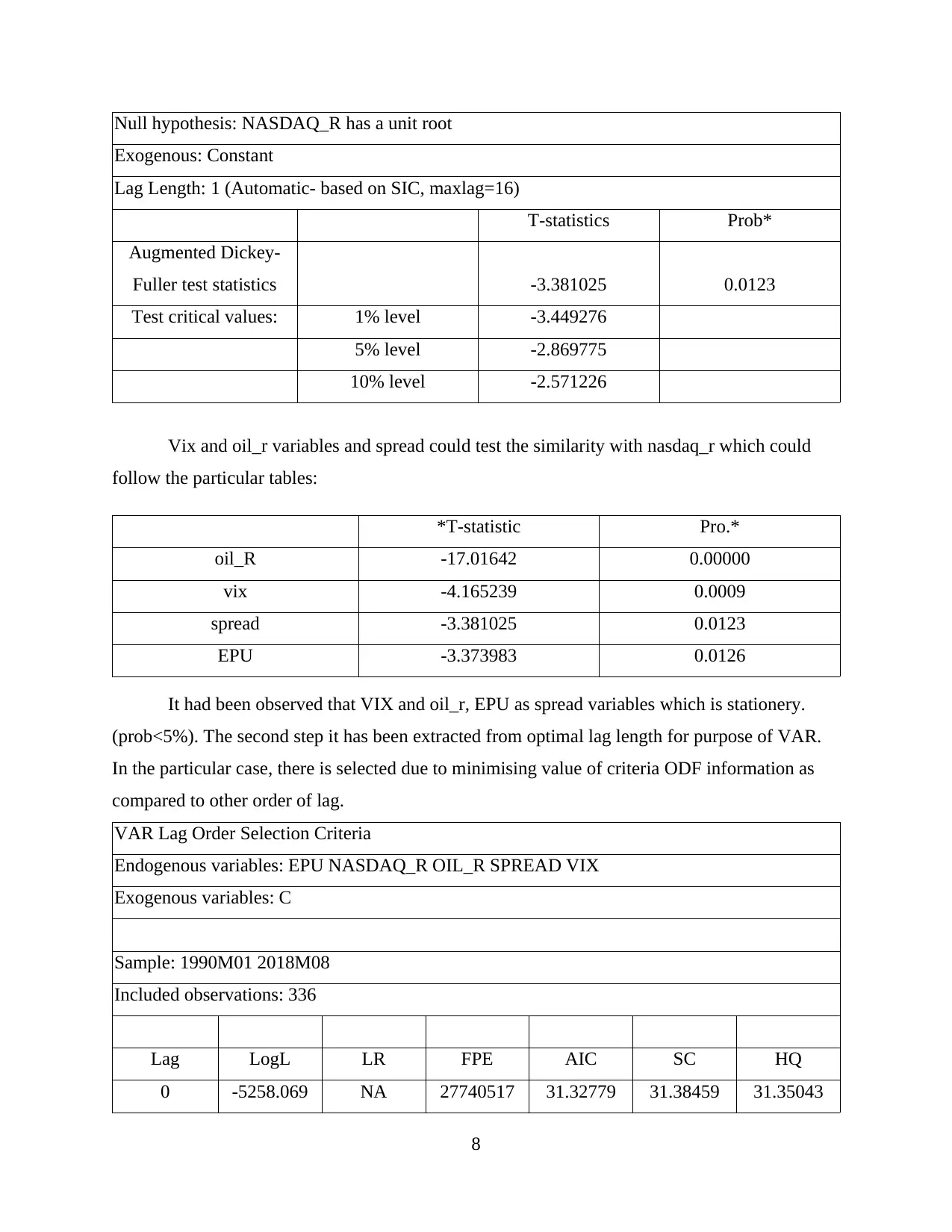
The first step is required for testing that every variables as stationery or non stationery
with application Dickey-Fuller unit root test. It could be observed that prob* which is less than
5%. Moreover, P value could be reject that hypothesis and nasdaq_q is stationery.
7

Null hypothesis: NASDAQ_R has a unit root
Exogenous: Constant
Lag Length: 1 (Automatic- based on SIC, maxlag=16)
T-statistics Prob*
Augmented Dickey-
Fuller test statistics -3.381025 0.0123
Test critical values: 1% level -3.449276
5% level -2.869775
10% level -2.571226
Vix and oil_r variables and spread could test the similarity with nasdaq_r which could
follow the particular tables:
*T-statistic Pro.*
oil_R -17.01642 0.00000
vix -4.165239 0.0009
spread -3.381025 0.0123
EPU -3.373983 0.0126
It had been observed that VIX and oil_r, EPU as spread variables which is stationery.
(prob<5%). The second step it has been extracted from optimal lag length for purpose of VAR.
In the particular case, there is selected due to minimising value of criteria ODF information as
compared to other order of lag.
VAR Lag Order Selection Criteria
Endogenous variables: EPU NASDAQ_R OIL_R SPREAD VIX
Exogenous variables: C
Sample: 1990M01 2018M08
Included observations: 336
Lag LogL LR FPE AIC SC HQ
0 -5258.069 NA 27740517 31.32779 31.38459 31.35043
8

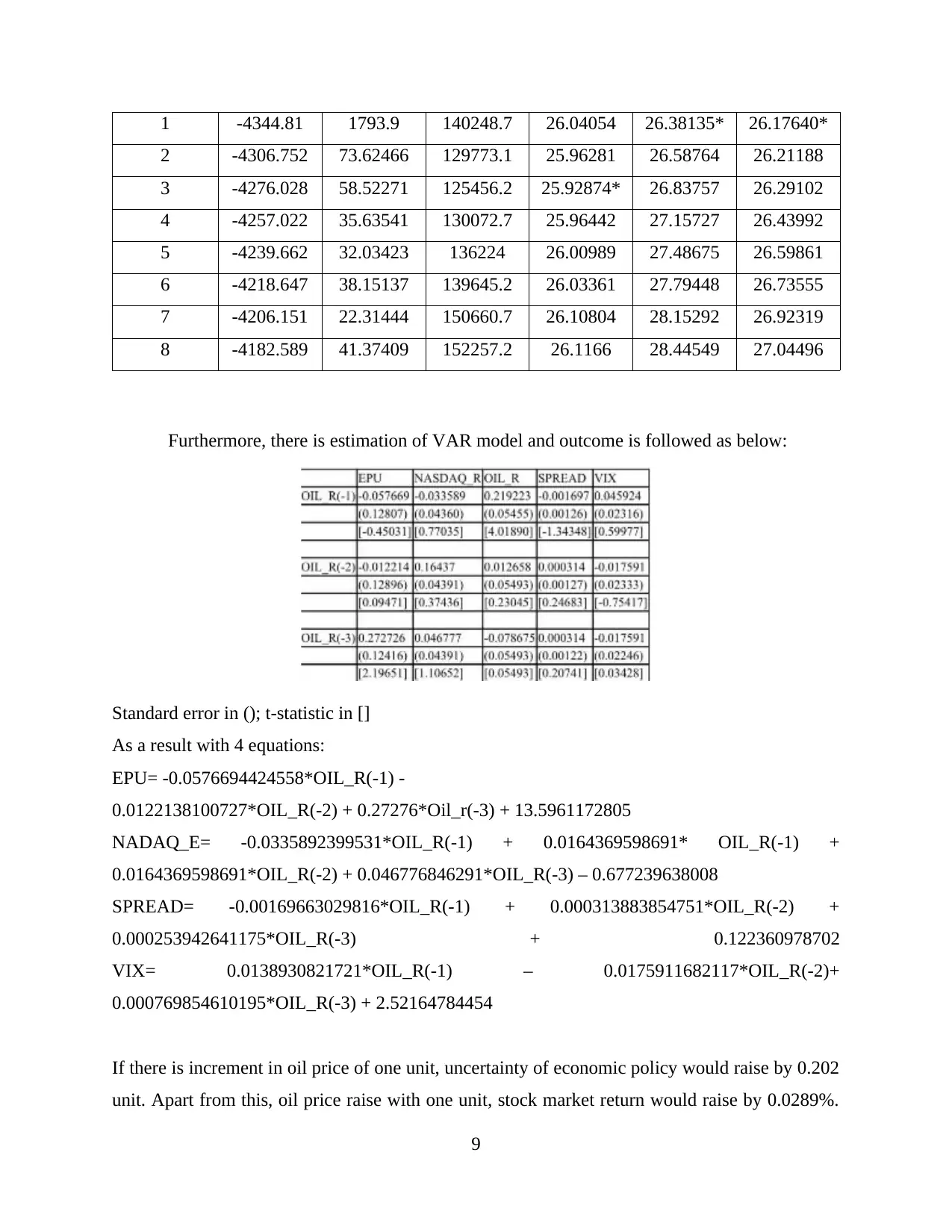
1 -4344.81 1793.9 140248.7 26.04054 26.38135* 26.17640*
2 -4306.752 73.62466 129773.1 25.96281 26.58764 26.21188
3 -4276.028 58.52271 125456.2 25.92874* 26.83757 26.29102
4 -4257.022 35.63541 130072.7 25.96442 27.15727 26.43992
5 -4239.662 32.03423 136224 26.00989 27.48675 26.59861
6 -4218.647 38.15137 139645.2 26.03361 27.79448 26.73555
7 -4206.151 22.31444 150660.7 26.10804 28.15292 26.92319
8 -4182.589 41.37409 152257.2 26.1166 28.44549 27.04496
Furthermore, there is estimation of VAR model and outcome is followed as below:
Standard error in (); t-statistic in []
As a result with 4 equations:
EPU= -0.0576694424558*OIL_R(-1) -
0.0122138100727*OIL_R(-2) + 0.27276*Oil_r(-3) + 13.5961172805
NADAQ_E= -0.0335892399531*OIL_R(-1) + 0.0164369598691* OIL_R(-1) +
0.0164369598691*OIL_R(-2) + 0.046776846291*OIL_R(-3) – 0.677239638008
SPREAD= -0.00169663029816*OIL_R(-1) + 0.000313883854751*OIL_R(-2) +
0.000253942641175*OIL_R(-3) + 0.122360978702
VIX= 0.0138930821721*OIL_R(-1) – 0.0175911682117*OIL_R(-2)+
0.000769854610195*OIL_R(-3) + 2.52164784454
If there is increment in oil price of one unit, uncertainty of economic policy would raise by 0.202
unit. Apart from this, oil price raise with one unit, stock market return would raise by 0.0289%.
9

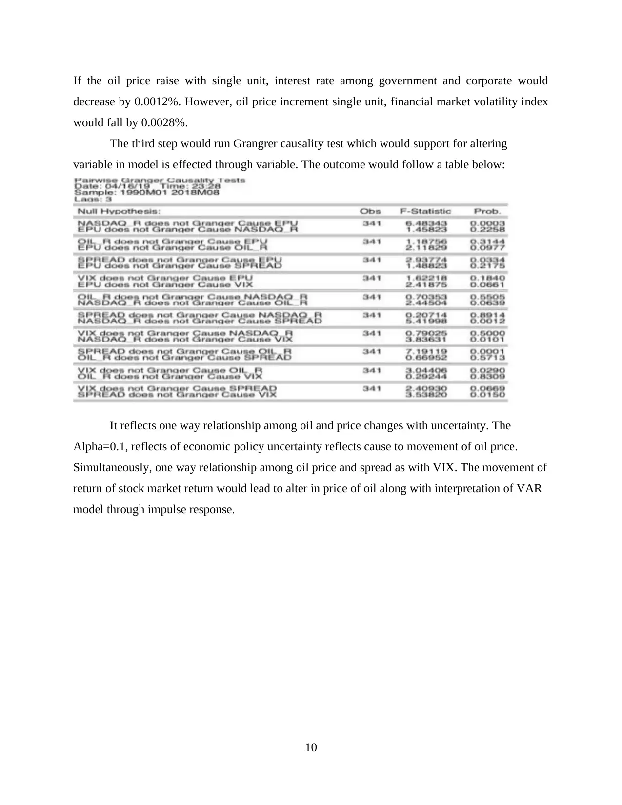
If the oil price raise with single unit, interest rate among government and corporate would
decrease by 0.0012%. However, oil price increment single unit, financial market volatility index
would fall by 0.0028%.
The third step would run Grangrer causality test which would support for altering
variable in model is effected through variable. The outcome would follow a table below:
It reflects one way relationship among oil and price changes with uncertainty. The
Alpha=0.1, reflects of economic policy uncertainty reflects cause to movement of oil price.
Simultaneously, one way relationship among oil price and spread as with VIX. The movement of
return of stock market return would lead to alter in price of oil along with interpretation of VAR
model through impulse response.
10