Detailed Project: Valuation, Hedging, and Option Strategies in Finance

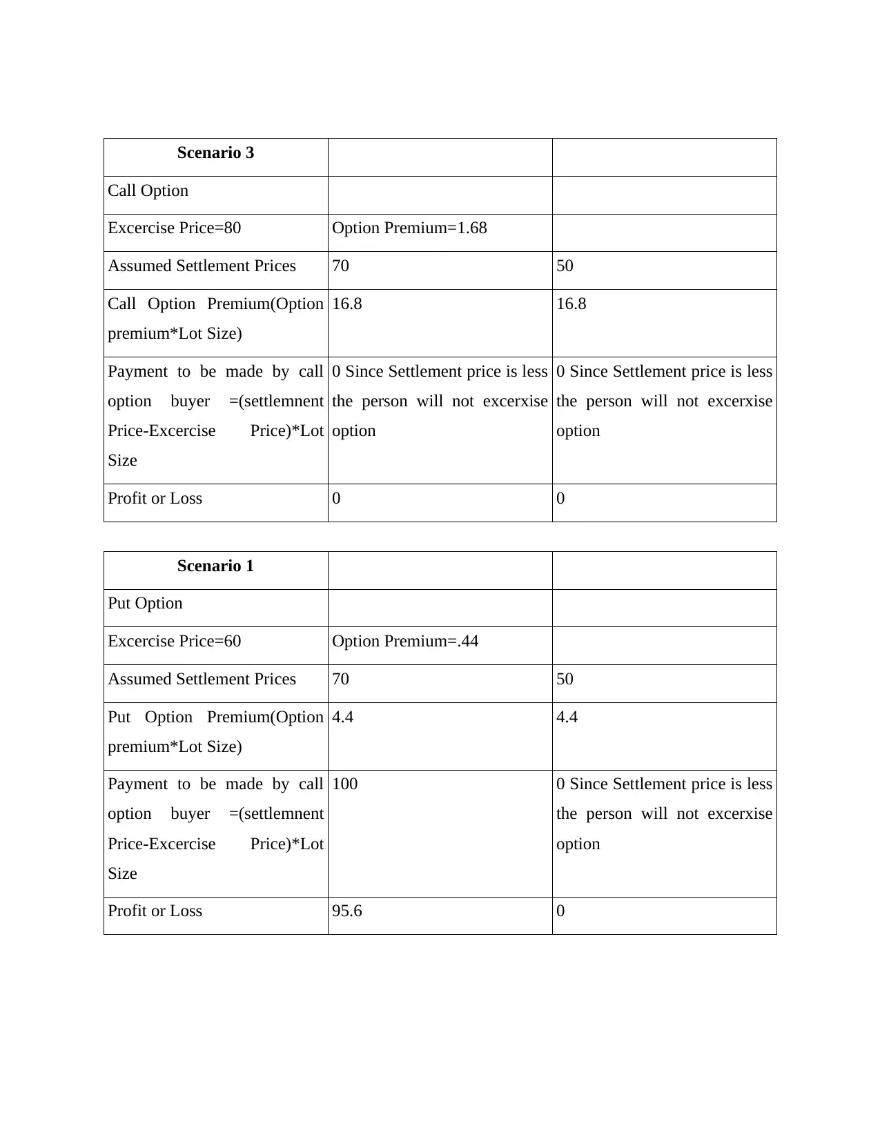
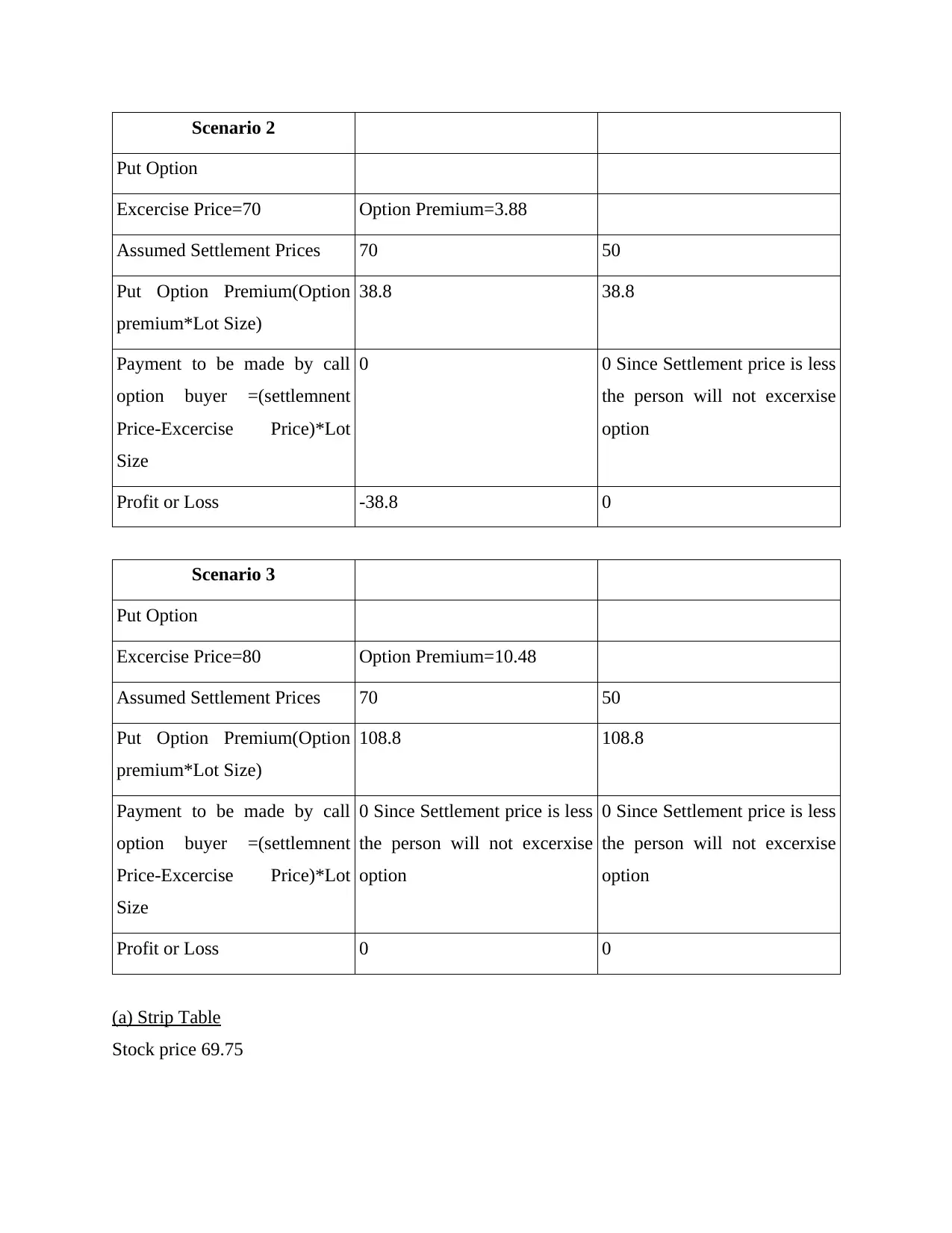
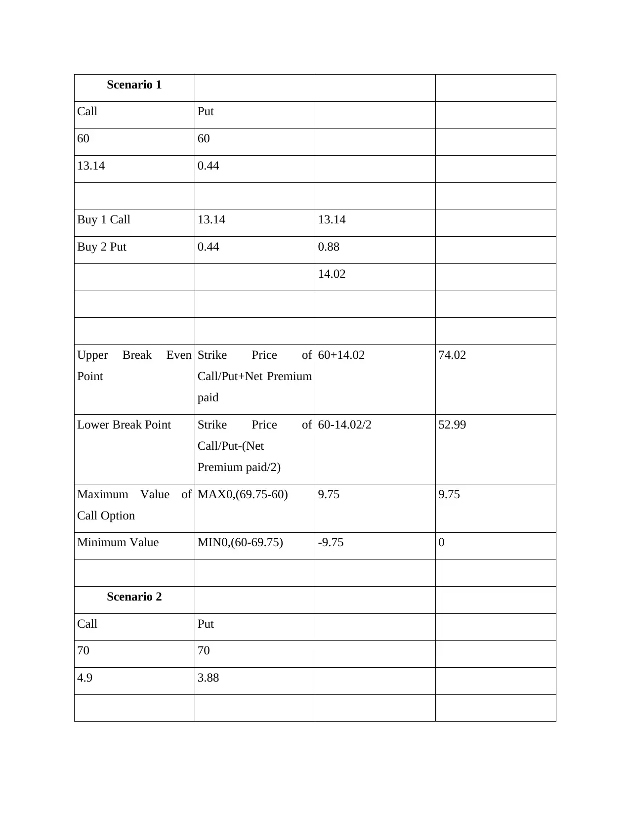
This finance project delves into various aspects of financial instruments and their applications. It begins with the calculation of continuously compounded zero rates using the bootstrap method and the determination of six-month forward rates. The project explores the use of zero rates and zero curves, bond pricing methodologies, and the analysis of the relationship between bond prices and yields, including hedging strategies. Furthermore, it includes a detailed analysis of option strategies, such as profit and loss statements for different scenarios. The project also covers the valuation of European put options using a four-step binomial tree and the Black-Scholes model, along with an explanation of the differences between American and European options. Finally, it explores the calculation of implied volatility and the hedging of a portfolio, including parallel and non-parallel shifts in the yield curve. The project also addresses the impacts of market movements on a portfolio and various option strategies like strip tables, reverse butterflies, straddles, and straps.

PROJECT

TABLE OF CONTENTS
QUESTION 1...................................................................................................................................1
A). Implicating Bootstrap method to calculate continuously compounded zero rates................1
B). Calculating the six months continuously compounded forward rates...................................1
C). Describing the one use for measuring the zero-rates and Zero curve....................................1
D). Measuring the price of bonds................................................................................................1
E). Measuring the price of bond.................................................................................................2
F). Analysing the direct and inverse relationship between bond prices and bond yield..............2
G) Hedging portfolio....................................................................................................................2
QUESTION 2...................................................................................................................................4
QUESTION 3...................................................................................................................................6
Profit and Loss Statement in case of Options..............................................................................6
(a) Strip Table..............................................................................................................................9
b)Reverse Butterfly....................................................................................................................11
c)Straddle...................................................................................................................................12
d)Strap........................................................................................................................................14
QUESTION 4.................................................................................................................................16
4.A Calculating four step binomial tree for European six month put option.............................16
4.B Estimating value of European six month put option with application of Black Scholes
model..........................................................................................................................................17
4 C Explaining reason American option differs from European option price...........................18
4 D Calculating implied volatility for future option on silver...................................................18
.......................................................................................................................................................20

QUESTION 1
A). Implicating Bootstrap method to calculate continuously compounded zero rates
n
Bond
price
[C]
ZC rate
of
maturity
[R]
Present
value
0.50 98 0% 98
1 104 8% 96.2963
Theoretical price of
bond 194.296
maturity period
Annual
coupon
Price of
security rate
0.5 0 98 -0.9796
1 8 104 -0.0385
B). Calculating the six months continuously compounded forward rates
FWD spot rate (1+ interest rate of variable currency) *days/ annual
base)
(1+ interest rate of base currency) *days/ annual base)
6 months -47.826 -98%
48.8219
12 months -3.7457 -4%
97.29
C). Describing the one use for measuring the zero-rates and Zero curve
As per ascertaining this bootstrapping method, on which it can be said that such operations
will be used as a reminder. Therefore, the xero coupon rate is a yield of an instrument which
does not generate any cash flow which is among date of issuance as well as maturity.
D). Measuring the price of bonds
Annual coupon (semi-annual) 10
yield to maturity 4%
time to maturity 2
face value 100

Bond price (C/1+i) ^2
Price of coupon $111.42
coupon days 180
net coupon days 180
number of coupons 4
E). Measuring the price of bond
Annual coupon (semi-
annual) 10
yield to maturity 2%
time to maturity 2
face value 100
Bond price (C/1+i) ^2
Price of coupon $115.61
coupon days 180
net coupon days 180
number of coupons 4
F). Analysing the direct and inverse relationship between bond prices and bond yield
In accordance with determining the direct or inverse relationship among bond yield and
bond prices it can be said that, they are promises which assist an individual for paying back
principles when loan is due.
Inverse relationship:
In this case, the bonds were issued and carried on a coupon rate which is akin to the market
interest rates. Therefore, in such circumstances there will be inverse relationship between interest
rates and bond prices. However, when the yield rate was 4% than the price of coupon was
$111.42. Similarly, when the yield was 2% per annum than the price of coupon was $115.61.
These are the value which is beyond the face value of bonds therefore, there will be no inverse
relationship among such variables.
G) Hedging portfolio
1.
Details Equity Bonds
Price of futures 94,062.50 94,062.50

contract
contract multiplier 60 20
Notional value 5643750 1881250
Value at risk 80000000 80000000
Hedge ratio 14.17 42.52
Position
value in 7.1
years Equity Bonds
long position of
futures S7.1 60000000(7.1) 426000000 20000000(7.1) 142000000
Short forward
position F-S7.1
94062.5-
60(7.1)
-
425905938
94062.5-
20(7.1)
-
141905938
Net payoff F 94062.5 94062.5 94062.5 94062.5
2. Treasury bond future position:
long position of futures 20500000(7.1) 145550000
Short forward position 96704.80-20500000(7.1) -145453295
Net payoff 96704.8 96704.8
3. Total hedge position:
In relation with ascertain the bond value gains or losses from the analysis on which it can be
said that, there have been implication of various formulas which is based on defining the
accurate outcomes. Therefore, the long position of bond is being analysed when the value was
$200000000 such as $142000000. In relation with analysing the short forward position on which
it has been analysed as -$141905938.
Moreover, as per changes in the bond value as $20500000 and in future prices which is
$96704.80. Thus, on the basis of such variations in the prices the long position of futures has
been anlsyed for bonds as $145550000 and short forward position for -$145453295.
4. Bond yield on bond portfolio:
Loss or gains have been made on treasury bond futures position:
If the yield of bond would have been increased on 30th September 2018 instead of 1st
February 2019. Thus, there will be losses on the treasury bond futures position.
Loss or gains have been made on bond portfolio:

If the yield of bond would have been increased on 30th September 2018 instead of 1st
February 2019. There will be gains in the bond portfolio.
Commenting of hedge outcomes:
As per analysing the hedge outcomes on which it can be said that, there has been changes in
the variables on which value of equity and bonds has been considered for having appropriate
determination of operational wants.
5. Parallel and non-parallel shift:
In accordance with the shift of yield curve on a parallel direction which defines relationship
between long term, short term and intermediate interest rates. Therefore, it determines that, it is a
normal outcome in market conditions. Therefore, in this case the parallel shift in yield curve
which in turn affects the fixed income maturities in short, long and intermediate interest.
Moreover, in analysing the non-parallel shift in yield curve of interest rates which
determines that, changes in the curve of bonds which do not occur evenly.
QUESTION 2
Name No. of
Shares
Average
Price
Total
Amount
Stop
Loss
Total
amout
After
stop loss
Loss Beta Risk
Free
Rate
Harrison 1500000 50 7500000
0
40 6000000
0
1500000
0
1.3 1.00%
Jack li 1500000 50 7500000
0
40 6000000
0
1500000
0
1.3 1.00%
Kieran 1500000 50 7500000
0
40 6000000
0
1500000
0
1.3 1.00%
Hoang 1500000 50 7500000
0
40 6000000
0
1500000
0
1.3 1.00%
Zhang 1500000 50 7500000
0
40 6000000
0
1500000
0
1.3 1.00%

(a)CAPM 0.01+1.3*(0.042-0.01) 5.16%
As to cover loss of 15000000
there is need for hedging
portfolio.
As in near future it be seen that
after 3 months there is
expected rise in the value of
portfolio so they can invest
more in same portfolio.
(b)So, as the return volatility dividend yield
are constant they should invest in same
portfolio
TodaY Share Price 50
After 3 months expected price 55
Profit 5
Loss amount 15000000
No.of shares to be purchased 3000000
Total Amount to be invested 150000000
(c)
If S&P 500 decreases
by 25%
Decrease 25%
Today Value 2700 675 2025
TodaY Share Price 50

(c)
Value of Share 37.5
Loss in Portfolio 12.5
No of Shares 1500000
Total amount of loss 18750000
(d)If S&P 500 decreases 10 1500
Today Value of Index 2700
TodaY Share Price 50
If Index 1500
Then Share Value 27.8
No of Shares 1500000
Total amount of loss 41666666.7
(e) If S&P 500
incerases by 15%
Today Value 2700 405 3105
TodaY Share Price 50
Value of Share 57.5
Profit in Portfolio 7.5
No of Shares 1500000
Total amount of loss 11250000

QUESTION 3
Profit and Loss Statement in case of Options
Assume Lot Size=10
Scenario 1
Call Option
Excercise Price=60 Option Premium=13.14
Assumed Settlement Prices 70 50
Call Option Premium(Option
premium*Lot Size)
131.4 131.4
Payment to be made by call
option buyer =(settlemnent
Price-Excercise Price)*Lot
Size
100 0 Since Settlement price is less
the person will not excerxise
option
Profit or Loss -31.4 0
Scenario 2
Call Option
Excercise Price=70 Option Premium=4.90
Assumed Settlement Prices 70 50
Call Option Premium(Option
premium*Lot Size)
49 49
Payment to be made by call
option buyer =(settlemnent
Price-Excercise Price)*Lot
Size
0 0 Since Settlement price is less
the person will not excerxise
option
Profit or Loss -49 0

Scenario 3
Call Option
Excercise Price=80 Option Premium=1.68
Assumed Settlement Prices 70 50
Call Option Premium(Option
premium*Lot Size)
16.8 16.8
Payment to be made by call
option buyer =(settlemnent
Price-Excercise Price)*Lot
Size
0 Since Settlement price is less
the person will not excerxise
option
0 Since Settlement price is less
the person will not excerxise
option
Profit or Loss 0 0
Scenario 1
Put Option
Excercise Price=60 Option Premium=.44
Assumed Settlement Prices 70 50
Put Option Premium(Option
premium*Lot Size)
4.4 4.4
Payment to be made by call
option buyer =(settlemnent
Price-Excercise Price)*Lot
Size
100 0 Since Settlement price is less
the person will not excerxise
option
Profit or Loss 95.6 0

Scenario 2
Put Option
Excercise Price=70 Option Premium=3.88
Assumed Settlement Prices 70 50
Put Option Premium(Option
premium*Lot Size)
38.8 38.8
Payment to be made by call
option buyer =(settlemnent
Price-Excercise Price)*Lot
Size
0 0 Since Settlement price is less
the person will not excerxise
option
Profit or Loss -38.8 0
Scenario 3
Put Option
Excercise Price=80 Option Premium=10.48
Assumed Settlement Prices 70 50
Put Option Premium(Option
premium*Lot Size)
108.8 108.8
Payment to be made by call
option buyer =(settlemnent
Price-Excercise Price)*Lot
Size
0 Since Settlement price is less
the person will not excerxise
option
0 Since Settlement price is less
the person will not excerxise
option
Profit or Loss 0 0
(a) Strip Table
Stock price 69.75

Scenario 1
Call Put
60 60
13.14 0.44
Buy 1 Call 13.14 13.14
Buy 2 Put 0.44 0.88
14.02
Upper Break Even
Point
Strike Price of
Call/Put+Net Premium
paid
60+14.02 74.02
Lower Break Point Strike Price of
Call/Put-(Net
Premium paid/2)
60-14.02/2 52.99
Maximum Value of
Call Option
MAX0,(69.75-60) 9.75 9.75
Minimum Value MIN0,(60-69.75) -9.75 0
Scenario 2
Call Put
70 70
4.9 3.88