EAS230 Engineering Computations Project: Finite Difference Modeling
VerifiedAdded on 2023/02/01
|15
|3221
|52
Project
AI Summary
This project report details a programming project for EAS230 Engineering Computations, focusing on modeling heat transfer within a uranium plate using finite difference methods. The project utilizes MATLAB to implement both explicit and implicit finite difference schemes, estimating temperature distributions over time under varying boundary conditions. The report includes a comprehensive breakdown of tasks, code listings for both solvers, and results from two test cases, each exploring different initial conditions, heat generation rates, and boundary conditions (prescribed temperature, heat flux, convection, and insulated). The results are presented through plots of temperature profiles at various time points, accompanied by a discussion of the findings and a comparison of the two numerical methods. The project aims to provide an understanding of numerical methods for solving heat transfer problems and demonstrates the application of MATLAB in engineering analysis.
Project Title
EAS230 Engineering Computations
Spring 2019
Group Name
PARTNER #1 Full Name, Lab Section, and UBitName
PARTNER #2 Full Name, Lab Section, and UBitName
Part Description of the breakdown of tasks
Script file Member #1 wrote up most of this part, Member #2 contributed in this
way
Explicit solver
Implicit solver
Please list other groups/individual that you may have worked with:
Group name #1, individual #1, etc.
Paraphrase This Document
Need a fresh take? Get an instant paraphrase of this document with our AI Paraphraser
EAS230 Spring 2019 Programming Project
GroupName: insert GroupName here
Table of Contents
Add your table of contents including each section number, title, and corresponding page
number
List of Tables and Figures
Add your list of tables and figures including each table number, title, and corresponding
page number and each figure number, title, and corresponding page number
Page 2 of 15
EAS 230 – Spring 2019 – PP
EAS230 Spring 2019 Programming Project
GroupName: insert GroupName here
1. Summary/Abstract
The finite difference methods are methods used to obtains approximate solutions for
temperature distributions across the plate and over time, T ( y ,u), at finite sets of x and t.
Different computer software has been used to determine and plotting the temperature
distributions across bodies such as MATLAB, python, etc.
In this project, MATLAB software is used to write programs that estimates the
temperature distribution across a large plate of uranium over time. Uranium plate generate
heat uniformly at a constant rate, the temperature distribution is approximated after
application of stated boundary conditions using finite difference numerical methods.
Page 3 of 15
EAS 230 – Spring 2019 – PP
⊘ This is a preview!⊘
Do you want full access?
Subscribe today to unlock all pages.
Trusted by 1+ million students worldwide
EAS230 Spring 2019 Programming Project
GroupName: insert GroupName here
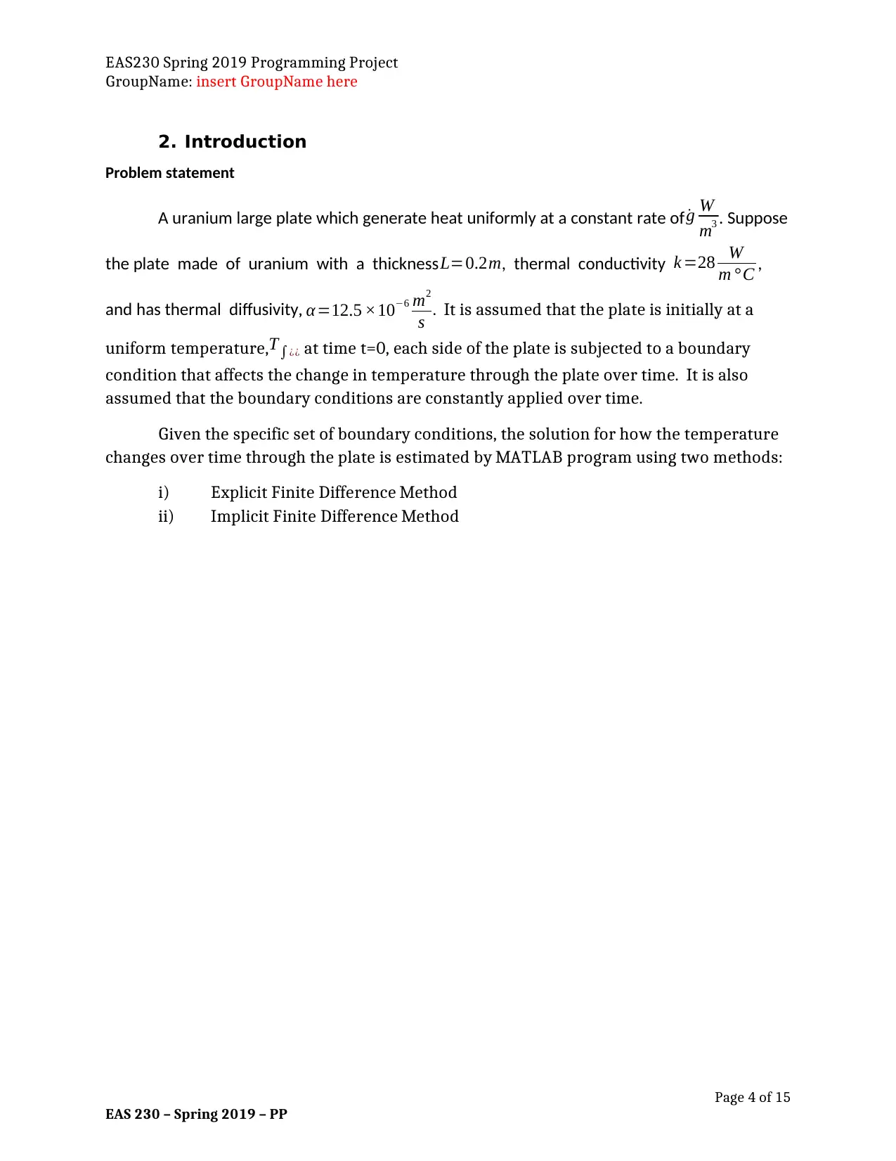
2. Introduction
Problem statement
A uranium large plate which generate heat uniformly at a constant rate of ˙g W
m3 . Suppose
the plate made of uranium with a thicknessL=0.2m, thermal conductivity k =28 W
m °C ,
and has thermal diffusivity, α=12.5 ×10⁻⁶ m2
s . It is assumed that the plate is initially at a
uniform temperature,T∫¿¿ at time t=0, each side of the plate is subjected to a boundary
condition that affects the change in temperature through the plate over time. It is also
assumed that the boundary conditions are constantly applied over time.
Given the specific set of boundary conditions, the solution for how the temperature
changes over time through the plate is estimated by MATLAB program using two methods:
i) Explicit Finite Difference Method
ii) Implicit Finite Difference Method
Page 4 of 15
EAS 230 – Spring 2019 – PP
GroupName: insert GroupName here
2. Introduction
Problem statement
A uranium large plate which generate heat uniformly at a constant rate of ˙g W
m3 . Suppose
the plate made of uranium with a thicknessL=0.2m, thermal conductivity k =28 W
m °C ,
and has thermal diffusivity, α=12.5 ×10⁻⁶ m2
s . It is assumed that the plate is initially at a
uniform temperature,T∫¿¿ at time t=0, each side of the plate is subjected to a boundary
condition that affects the change in temperature through the plate over time. It is also
assumed that the boundary conditions are constantly applied over time.
Given the specific set of boundary conditions, the solution for how the temperature
changes over time through the plate is estimated by MATLAB program using two methods:
i) Explicit Finite Difference Method
ii) Implicit Finite Difference Method
Page 4 of 15
EAS 230 – Spring 2019 – PP
Paraphrase This Document
Need a fresh take? Get an instant paraphrase of this document with our AI Paraphraser
EAS230 Spring 2019 Programming Project
GroupName: insert GroupName here
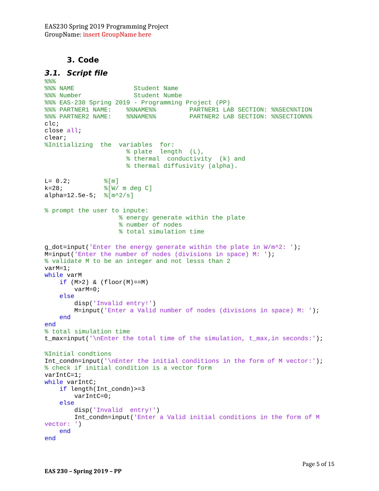
3. Code
3.1. Script file
%%%
%%% NAME Student Name
%%% Number Student Numbe
%%% EAS-230 Spring 2019 - Programming Project (PP)
%%% PARTNER1 NAME: %%NAME%% PARTNER1 LAB SECTION: %%SEC%%TION
%%% PARTNER2 NAME: %%NAME%% PARTNER2 LAB SECTION: %%SECTION%%
clc;
close all;
clear;
%Initializing the variables for:
% plate length (L),
% thermal conductivity (k) and
% thermal diffusivity (alpha).
L= 0.2; %[m]
k=28; %[W/ m deg C]
alpha=12.5e-5; %[m^2/s]
% prompt the user to inpute:
% energy generate within the plate
% number of nodes
% total simulation time
g_dot=input('Enter the energy generate within the plate in W/m^2: ');
M=input('Enter the number of nodes (divisions in space) M: ');
% validate M to be an integer and not lesss than 2
varM=1;
while varM
if (M>2) & (floor(M)==M)
varM=0;
else
disp('Invalid entry!')
M=input('Enter a Valid number of nodes (divisions in space) M: ');
end
end
% total simulation time
t_max=input('\nEnter the total time of the simulation, t_max,in seconds:');
%Initial condtions
Int_condn=input('\nEnter the initial conditions in the form of M vector:');
% check if initial condition is a vector form
varIntC=1;
while varIntC;
if length(Int_condn)>=3
varIntC=0;
else
disp('Invalid entry!')
Int_condn=input('Enter a Valid initial conditions in the form of M
vector: ')
end
end
Page 5 of 15
EAS 230 – Spring 2019 – PP
GroupName: insert GroupName here
3. Code
3.1. Script file
%%%
%%% NAME Student Name
%%% Number Student Numbe
%%% EAS-230 Spring 2019 - Programming Project (PP)
%%% PARTNER1 NAME: %%NAME%% PARTNER1 LAB SECTION: %%SEC%%TION
%%% PARTNER2 NAME: %%NAME%% PARTNER2 LAB SECTION: %%SECTION%%
clc;
close all;
clear;
%Initializing the variables for:
% plate length (L),
% thermal conductivity (k) and
% thermal diffusivity (alpha).
L= 0.2; %[m]
k=28; %[W/ m deg C]
alpha=12.5e-5; %[m^2/s]
% prompt the user to inpute:
% energy generate within the plate
% number of nodes
% total simulation time
g_dot=input('Enter the energy generate within the plate in W/m^2: ');
M=input('Enter the number of nodes (divisions in space) M: ');
% validate M to be an integer and not lesss than 2
varM=1;
while varM
if (M>2) & (floor(M)==M)
varM=0;
else
disp('Invalid entry!')
M=input('Enter a Valid number of nodes (divisions in space) M: ');
end
end
% total simulation time
t_max=input('\nEnter the total time of the simulation, t_max,in seconds:');
%Initial condtions
Int_condn=input('\nEnter the initial conditions in the form of M vector:');
% check if initial condition is a vector form
varIntC=1;
while varIntC;
if length(Int_condn)>=3
varIntC=0;
else
disp('Invalid entry!')
Int_condn=input('Enter a Valid initial conditions in the form of M
vector: ')
end
end
Page 5 of 15
EAS 230 – Spring 2019 – PP
EAS230 Spring 2019 Programming Project
GroupName: insert GroupName here
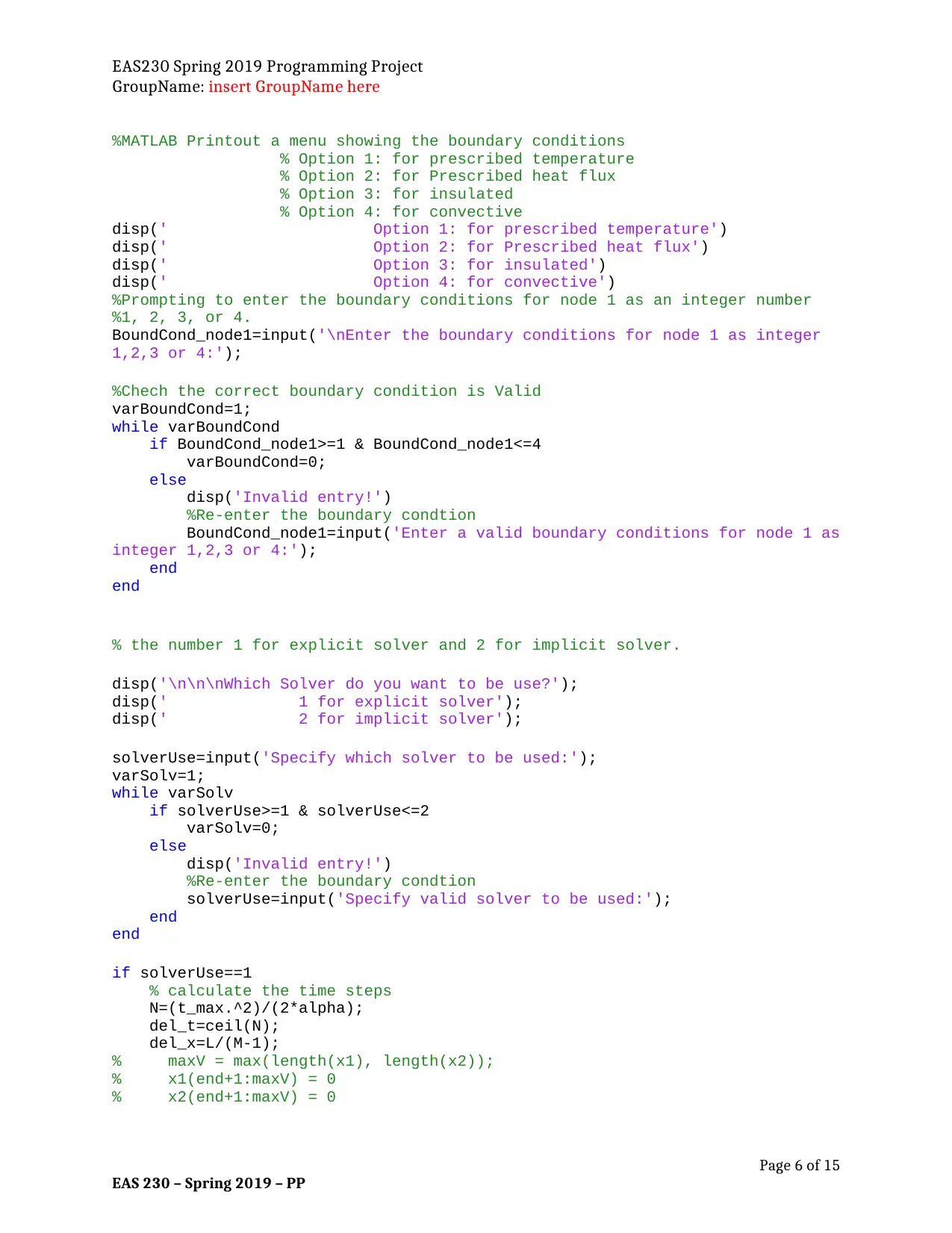
%MATLAB Printout a menu showing the boundary conditions
% Option 1: for prescribed temperature
% Option 2: for Prescribed heat flux
% Option 3: for insulated
% Option 4: for convective
disp(' Option 1: for prescribed temperature')
disp(' Option 2: for Prescribed heat flux')
disp(' Option 3: for insulated')
disp(' Option 4: for convective')
%Prompting to enter the boundary conditions for node 1 as an integer number
%1, 2, 3, or 4.
BoundCond_node1=input('\nEnter the boundary conditions for node 1 as integer
1,2,3 or 4:');
%Chech the correct boundary condition is Valid
varBoundCond=1;
while varBoundCond
if BoundCond_node1>=1 & BoundCond_node1<=4
varBoundCond=0;
else
disp('Invalid entry!')
%Re-enter the boundary condtion
BoundCond_node1=input('Enter a valid boundary conditions for node 1 as
integer 1,2,3 or 4:');
end
end
% the number 1 for explicit solver and 2 for implicit solver.
disp('\n\n\nWhich Solver do you want to be use?');
disp(' 1 for explicit solver');
disp(' 2 for implicit solver');
solverUse=input('Specify which solver to be used:');
varSolv=1;
while varSolv
if solverUse>=1 & solverUse<=2
varSolv=0;
else
disp('Invalid entry!')
%Re-enter the boundary condtion
solverUse=input('Specify valid solver to be used:');
end
end
if solverUse==1
% calculate the time steps
N=(t_max.^2)/(2*alpha);
del_t=ceil(N);
del_x=L/(M-1);
% maxV = max(length(x1), length(x2));
% x1(end+1:maxV) = 0
% x2(end+1:maxV) = 0
Page 6 of 15
EAS 230 – Spring 2019 – PP
GroupName: insert GroupName here
%MATLAB Printout a menu showing the boundary conditions
% Option 1: for prescribed temperature
% Option 2: for Prescribed heat flux
% Option 3: for insulated
% Option 4: for convective
disp(' Option 1: for prescribed temperature')
disp(' Option 2: for Prescribed heat flux')
disp(' Option 3: for insulated')
disp(' Option 4: for convective')
%Prompting to enter the boundary conditions for node 1 as an integer number
%1, 2, 3, or 4.
BoundCond_node1=input('\nEnter the boundary conditions for node 1 as integer
1,2,3 or 4:');
%Chech the correct boundary condition is Valid
varBoundCond=1;
while varBoundCond
if BoundCond_node1>=1 & BoundCond_node1<=4
varBoundCond=0;
else
disp('Invalid entry!')
%Re-enter the boundary condtion
BoundCond_node1=input('Enter a valid boundary conditions for node 1 as
integer 1,2,3 or 4:');
end
end
% the number 1 for explicit solver and 2 for implicit solver.
disp('\n\n\nWhich Solver do you want to be use?');
disp(' 1 for explicit solver');
disp(' 2 for implicit solver');
solverUse=input('Specify which solver to be used:');
varSolv=1;
while varSolv
if solverUse>=1 & solverUse<=2
varSolv=0;
else
disp('Invalid entry!')
%Re-enter the boundary condtion
solverUse=input('Specify valid solver to be used:');
end
end
if solverUse==1
% calculate the time steps
N=(t_max.^2)/(2*alpha);
del_t=ceil(N);
del_x=L/(M-1);
% maxV = max(length(x1), length(x2));
% x1(end+1:maxV) = 0
% x2(end+1:maxV) = 0
Page 6 of 15
EAS 230 – Spring 2019 – PP
⊘ This is a preview!⊘
Do you want full access?
Subscribe today to unlock all pages.
Trusted by 1+ million students worldwide
EAS230 Spring 2019 Programming Project
GroupName: insert GroupName here
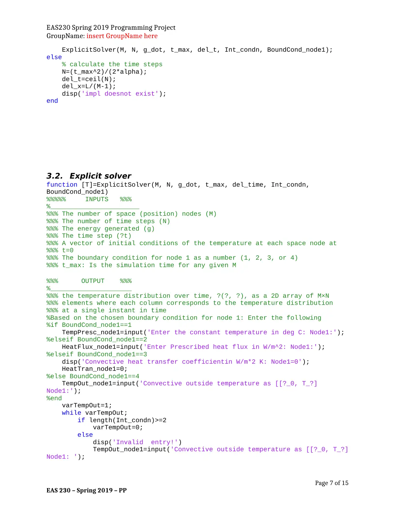
ExplicitSolver(M, N, g_dot, t_max, del_t, Int_condn, BoundCond_node1);
else
% calculate the time steps
N=(t_max^2)/(2*alpha);
del_t=ceil(N);
del_x=L/(M-1);
disp('impl doesnot exist');
end
3.2. Explicit solver
function [T]=ExplicitSolver(M, N, g_dot, t_max, del_time, Int_condn,
BoundCond_node1)
%%%%% INPUTS %%%
%_______________________
%%% The number of space (position) nodes (M)
%%% The number of time steps (N)
%%% The energy generated (g)
%%% The time step (?t)
%%% A vector of initial conditions of the temperature at each space node at
%%% t=0
%%% The boundary condition for node 1 as a number (1, 2, 3, or 4)
%%% t_max: Is the simulation time for any given M
%%% OUTPUT %%%
%_____________________
%%% the temperature distribution over time, ?(?, ?), as a 2D array of M×N
%%% elements where each column corresponds to the temperature distribution
%%% at a single instant in time
%Based on the chosen boundary condition for node 1: Enter the following
%if BoundCond_node1==1
TempPresc_node1=input('Enter the constant temperature in deg C: Node1:');
%elseif BoundCond_node1==2
HeatFlux_node1=input('Enter Prescribed heat flux in W/m^2: Node1:');
%elseif BoundCond_node1==3
disp('Convective heat transfer coefficientin W/m*2 K: Node1=0');
HeatTran_node1=0;
%else BoundCond_node1==4
TempOut_node1=input('Convective outside temperature as [[?_0, T_?]
Node1:');
%end
varTempOut=1;
while varTempOut;
if length(Int_condn)>=2
varTempOut=0;
else
disp('Invalid entry!')
TempOut_node1=input('Convective outside temperature as [[?_0, T_?]
Node1: ');
Page 7 of 15
EAS 230 – Spring 2019 – PP
GroupName: insert GroupName here
ExplicitSolver(M, N, g_dot, t_max, del_t, Int_condn, BoundCond_node1);
else
% calculate the time steps
N=(t_max^2)/(2*alpha);
del_t=ceil(N);
del_x=L/(M-1);
disp('impl doesnot exist');
end
3.2. Explicit solver
function [T]=ExplicitSolver(M, N, g_dot, t_max, del_time, Int_condn,
BoundCond_node1)
%%%%% INPUTS %%%
%_______________________
%%% The number of space (position) nodes (M)
%%% The number of time steps (N)
%%% The energy generated (g)
%%% The time step (?t)
%%% A vector of initial conditions of the temperature at each space node at
%%% t=0
%%% The boundary condition for node 1 as a number (1, 2, 3, or 4)
%%% t_max: Is the simulation time for any given M
%%% OUTPUT %%%
%_____________________
%%% the temperature distribution over time, ?(?, ?), as a 2D array of M×N
%%% elements where each column corresponds to the temperature distribution
%%% at a single instant in time
%Based on the chosen boundary condition for node 1: Enter the following
%if BoundCond_node1==1
TempPresc_node1=input('Enter the constant temperature in deg C: Node1:');
%elseif BoundCond_node1==2
HeatFlux_node1=input('Enter Prescribed heat flux in W/m^2: Node1:');
%elseif BoundCond_node1==3
disp('Convective heat transfer coefficientin W/m*2 K: Node1=0');
HeatTran_node1=0;
%else BoundCond_node1==4
TempOut_node1=input('Convective outside temperature as [[?_0, T_?]
Node1:');
%end
varTempOut=1;
while varTempOut;
if length(Int_condn)>=2
varTempOut=0;
else
disp('Invalid entry!')
TempOut_node1=input('Convective outside temperature as [[?_0, T_?]
Node1: ');
Page 7 of 15
EAS 230 – Spring 2019 – PP
Paraphrase This Document
Need a fresh take? Get an instant paraphrase of this document with our AI Paraphraser
EAS230 Spring 2019 Programming Project
GroupName: insert GroupName here
end
end
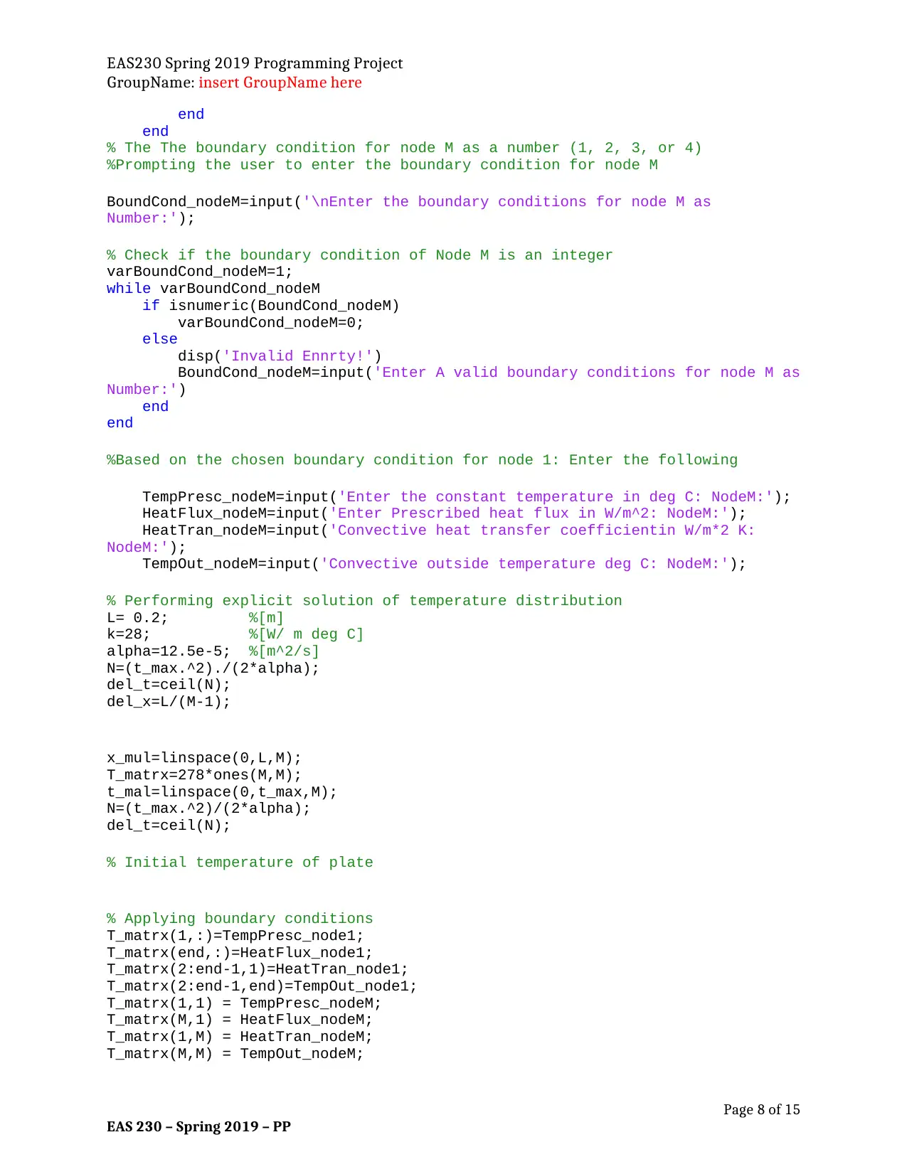
% The The boundary condition for node M as a number (1, 2, 3, or 4)
%Prompting the user to enter the boundary condition for node M
BoundCond_nodeM=input('\nEnter the boundary conditions for node M as
Number:');
% Check if the boundary condition of Node M is an integer
varBoundCond_nodeM=1;
while varBoundCond_nodeM
if isnumeric(BoundCond_nodeM)
varBoundCond_nodeM=0;
else
disp('Invalid Ennrty!')
BoundCond_nodeM=input('Enter A valid boundary conditions for node M as
Number:')
end
end
%Based on the chosen boundary condition for node 1: Enter the following
TempPresc_nodeM=input('Enter the constant temperature in deg C: NodeM:');
HeatFlux_nodeM=input('Enter Prescribed heat flux in W/m^2: NodeM:');
HeatTran_nodeM=input('Convective heat transfer coefficientin W/m*2 K:
NodeM:');
TempOut_nodeM=input('Convective outside temperature deg C: NodeM:');
% Performing explicit solution of temperature distribution
L= 0.2; %[m]
k=28; %[W/ m deg C]
alpha=12.5e-5; %[m^2/s]
N=(t_max.^2)./(2*alpha);
del_t=ceil(N);
del_x=L/(M-1);
x_mul=linspace(0,L,M);
T_matrx=278*ones(M,M);
t_mal=linspace(0,t_max,M);
N=(t_max.^2)/(2*alpha);
del_t=ceil(N);
% Initial temperature of plate
% Applying boundary conditions
T_matrx(1,:)=TempPresc_node1;
T_matrx(end,:)=HeatFlux_node1;
T_matrx(2:end-1,1)=HeatTran_node1;
T_matrx(2:end-1,end)=TempOut_node1;
T_matrx(1,1) = TempPresc_nodeM;
T_matrx(M,1) = HeatFlux_nodeM;
T_matrx(1,M) = HeatTran_nodeM;
T_matrx(M,M) = TempOut_nodeM;
Page 8 of 15
EAS 230 – Spring 2019 – PP
GroupName: insert GroupName here
end
end
% The The boundary condition for node M as a number (1, 2, 3, or 4)
%Prompting the user to enter the boundary condition for node M
BoundCond_nodeM=input('\nEnter the boundary conditions for node M as
Number:');
% Check if the boundary condition of Node M is an integer
varBoundCond_nodeM=1;
while varBoundCond_nodeM
if isnumeric(BoundCond_nodeM)
varBoundCond_nodeM=0;
else
disp('Invalid Ennrty!')
BoundCond_nodeM=input('Enter A valid boundary conditions for node M as
Number:')
end
end
%Based on the chosen boundary condition for node 1: Enter the following
TempPresc_nodeM=input('Enter the constant temperature in deg C: NodeM:');
HeatFlux_nodeM=input('Enter Prescribed heat flux in W/m^2: NodeM:');
HeatTran_nodeM=input('Convective heat transfer coefficientin W/m*2 K:
NodeM:');
TempOut_nodeM=input('Convective outside temperature deg C: NodeM:');
% Performing explicit solution of temperature distribution
L= 0.2; %[m]
k=28; %[W/ m deg C]
alpha=12.5e-5; %[m^2/s]
N=(t_max.^2)./(2*alpha);
del_t=ceil(N);
del_x=L/(M-1);
x_mul=linspace(0,L,M);
T_matrx=278*ones(M,M);
t_mal=linspace(0,t_max,M);
N=(t_max.^2)/(2*alpha);
del_t=ceil(N);
% Initial temperature of plate
% Applying boundary conditions
T_matrx(1,:)=TempPresc_node1;
T_matrx(end,:)=HeatFlux_node1;
T_matrx(2:end-1,1)=HeatTran_node1;
T_matrx(2:end-1,end)=TempOut_node1;
T_matrx(1,1) = TempPresc_nodeM;
T_matrx(M,1) = HeatFlux_nodeM;
T_matrx(1,M) = HeatTran_nodeM;
T_matrx(M,M) = TempOut_nodeM;
Page 8 of 15
EAS 230 – Spring 2019 – PP
EAS230 Spring 2019 Programming Project
GroupName: insert GroupName here
T_int=T_matrx;
tau=alpha*del_t/(del_x^2);
tic
for ki=[1 2.5 5 10]
T_int=T_matrx;
for ii=2:(M-1)
for ji=2:(M-1)
term_1=tau*T_int(ii-1, ji);
term_2=(1-tau)*T_int(ii, ji);
term_3=tau*(T_int(ii+1,ji));
term_4=tau*(g_dot*del_x^2)/k;
T_matrx(ii,ji)=T_int(ii,ji)+term_1+term_2+(term_3*term_4);
end
end
end
t_time=toc;
plot(T_matrx,X_x)
title('Explicit solver at M=201, differenr t_m_a_x');
xlabel('Temperature');
ylabel('Plate Thickness, x');
legend('t_m_a_x = 60 s', 't_m_a_x = 150 s', 't_m_a_x = 300 s', 't_m_a_x = 600
s', 'location', 'bestoutside');
end
3.3. Implicit solver
Lt the name of the function with a description of what the function does and how to use it.
You should include the mathematical functions and any pseudocode you used to solve the
problem and how it is solved.
Page 9 of 15
EAS 230 – Spring 2019 – PP
⊘ This is a preview!⊘
Do you want full access?
Subscribe today to unlock all pages.
Trusted by 1+ million students worldwide
EAS230 Spring 2019 Programming Project
GroupName: insert GroupName here
4. Results and discussion
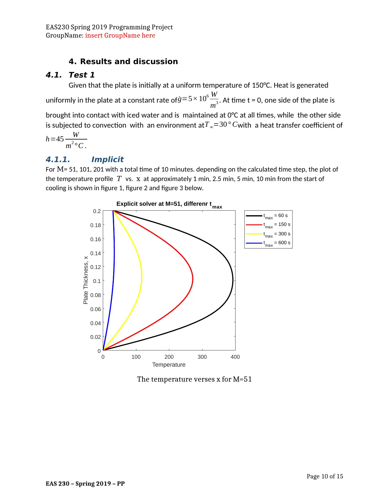
4.1. Test 1
Given that the plate is initially at a uniform temperature of 150°C. Heat is generated
uniformly in the plate at a constant rate of ˙g=5× 10⁶ W
m3 . At time t = 0, one side of the plate is
brought into contact with iced water and is maintained at 0°C at all times, while the other side
is subjected to convection with an environment at T ∞=30 ° Cwith a heat transfer coefficient of
h=45 W
m2 °C .
4.1.1. Implicit
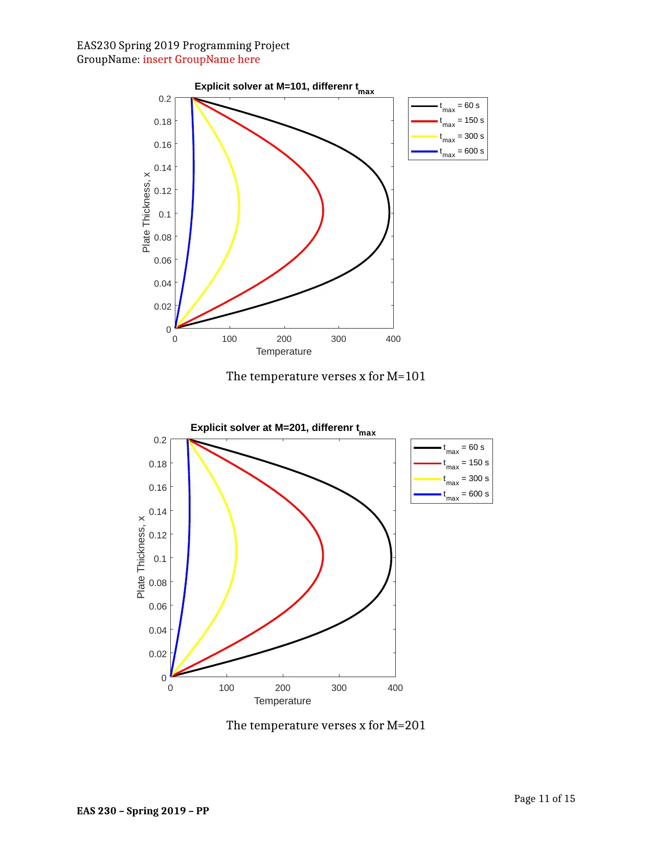
For M= 51, 101, 201 with a total time of 10 minutes. depending on the calculated time step, the plot of
the temperature profile 𝑇 vs. x at approximately 1 min, 2.5 min, 5 min, 10 min from the start of
cooling is shown in figure 1, figure 2 and figure 3 below.
0 100 200 300 400
Temperature
0
0.02
0.04
0.06
0.08
0.1
0.12
0.14
0.16
0.18
0.2
Plate Thickness, x
Explicit solver at M=51, differenr t max
tmax = 60 s
tmax = 150 s
tmax = 300 s
tmax = 600 s
The temperature verses x for M=51
Page 10 of 15
EAS 230 – Spring 2019 – PP
GroupName: insert GroupName here
4. Results and discussion
4.1. Test 1
Given that the plate is initially at a uniform temperature of 150°C. Heat is generated
uniformly in the plate at a constant rate of ˙g=5× 10⁶ W
m3 . At time t = 0, one side of the plate is
brought into contact with iced water and is maintained at 0°C at all times, while the other side
is subjected to convection with an environment at T ∞=30 ° Cwith a heat transfer coefficient of
h=45 W
m2 °C .
4.1.1. Implicit
For M= 51, 101, 201 with a total time of 10 minutes. depending on the calculated time step, the plot of
the temperature profile 𝑇 vs. x at approximately 1 min, 2.5 min, 5 min, 10 min from the start of
cooling is shown in figure 1, figure 2 and figure 3 below.
0 100 200 300 400
Temperature
0
0.02
0.04
0.06
0.08
0.1
0.12
0.14
0.16
0.18
0.2
Plate Thickness, x
Explicit solver at M=51, differenr t max
tmax = 60 s
tmax = 150 s
tmax = 300 s
tmax = 600 s
The temperature verses x for M=51
Page 10 of 15
EAS 230 – Spring 2019 – PP
Paraphrase This Document
Need a fresh take? Get an instant paraphrase of this document with our AI Paraphraser
EAS230 Spring 2019 Programming Project
GroupName: insert GroupName here
0 100 200 300 400
Temperature
0
0.02
0.04
0.06
0.08
0.1
0.12
0.14
0.16
0.18
0.2
Plate Thickness, x
Explicit solver at M=101, differenr tmax
tmax = 60 s
tmax = 150 s
tmax = 300 s
tmax = 600 s
The temperature verses x for M=101
0 100 200 300 400
Temperature
0
0.02
0.04
0.06
0.08
0.1
0.12
0.14
0.16
0.18
0.2
Plate Thickness, x
Explicit solver at M=201, differenr tmax
tmax = 60 s
tmax = 150 s
tmax = 300 s
tmax = 600 s
The temperature verses x for M=201
Page 11 of 15
EAS 230 – Spring 2019 – PP
EAS230 Spring 2019 Programming Project
GroupName: insert GroupName here
4.1.2. Explicit
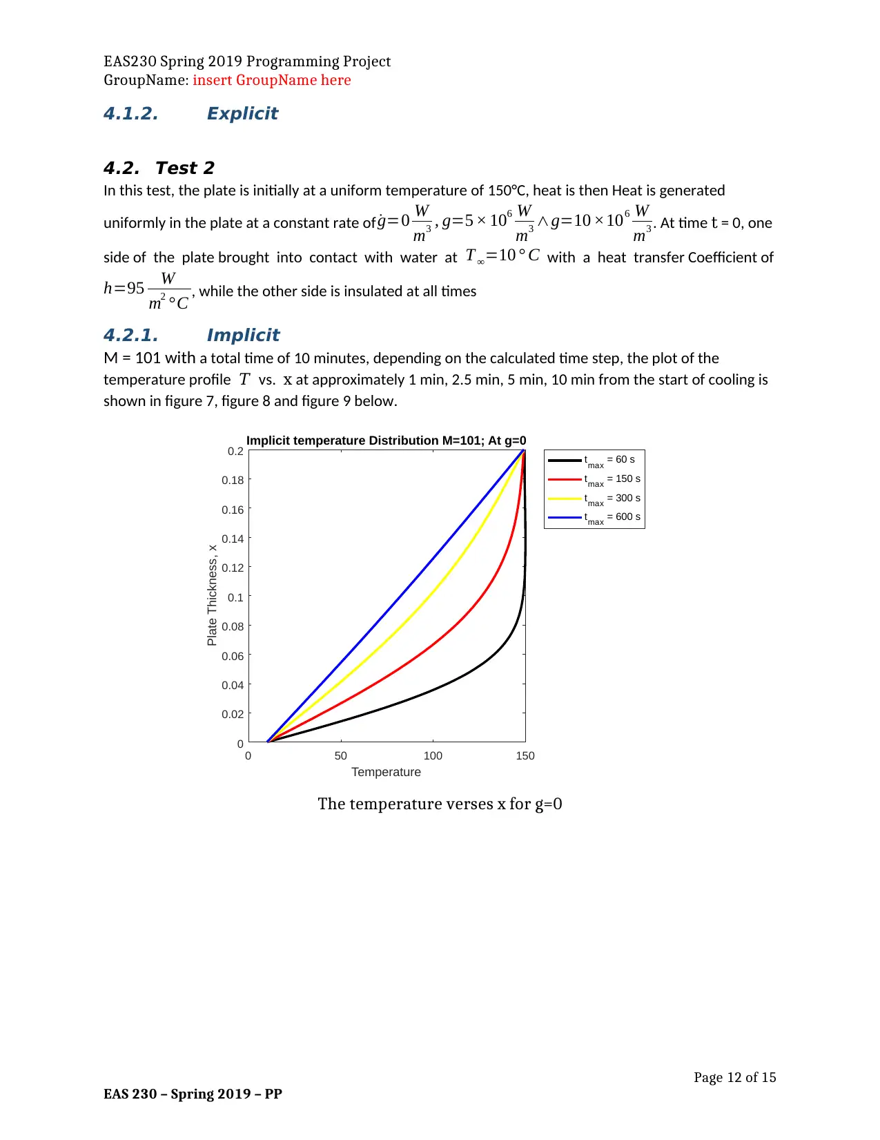
4.2. Test 2
In this test, the plate is initially at a uniform temperature of 150°C, heat is then Heat is generated
uniformly in the plate at a constant rate of ˙g=0 W
m3 , g=5 × 10⁶ W
m3 ∧g=10 ×106 W
m3 . At time t = 0, one
side of the plate brought into contact with water at T ∞=10 ° C with a heat transfer Coefficient of
h=95 W
m2 °C , while the other side is insulated at all times
4.2.1. Implicit
M = 101 with a total time of 10 minutes, depending on the calculated time step, the plot of the
temperature profile 𝑇 vs. x at approximately 1 min, 2.5 min, 5 min, 10 min from the start of cooling is
shown in figure 7, figure 8 and figure 9 below.
0 50 100 150
Temperature
0
0.02
0.04
0.06
0.08
0.1
0.12
0.14
0.16
0.18
0.2
Plate Thickness, x
Implicit temperature Distribution M=101; At g=0
tmax = 60 s
tmax = 150 s
tmax = 300 s
tmax = 600 s
The temperature verses x for g=0
Page 12 of 15
EAS 230 – Spring 2019 – PP
GroupName: insert GroupName here
4.1.2. Explicit
4.2. Test 2
In this test, the plate is initially at a uniform temperature of 150°C, heat is then Heat is generated
uniformly in the plate at a constant rate of ˙g=0 W
m3 , g=5 × 10⁶ W
m3 ∧g=10 ×106 W
m3 . At time t = 0, one
side of the plate brought into contact with water at T ∞=10 ° C with a heat transfer Coefficient of
h=95 W
m2 °C , while the other side is insulated at all times
4.2.1. Implicit
M = 101 with a total time of 10 minutes, depending on the calculated time step, the plot of the
temperature profile 𝑇 vs. x at approximately 1 min, 2.5 min, 5 min, 10 min from the start of cooling is
shown in figure 7, figure 8 and figure 9 below.
0 50 100 150
Temperature
0
0.02
0.04
0.06
0.08
0.1
0.12
0.14
0.16
0.18
0.2
Plate Thickness, x
Implicit temperature Distribution M=101; At g=0
tmax = 60 s
tmax = 150 s
tmax = 300 s
tmax = 600 s
The temperature verses x for g=0
Page 12 of 15
EAS 230 – Spring 2019 – PP
⊘ This is a preview!⊘
Do you want full access?
Subscribe today to unlock all pages.
Trusted by 1+ million students worldwide
1 out of 15

Your All-in-One AI-Powered Toolkit for Academic Success.
+13062052269
info@desklib.com
Available 24*7 on WhatsApp / Email
![[object Object]](/_next/static/media/star-bottom.7253800d.svg)
Unlock your academic potential
Copyright © 2020–2026 A2Z Services. All Rights Reserved. Developed and managed by ZUCOL.