FIR Filter Design and Implementation Assignment in Signal Processing

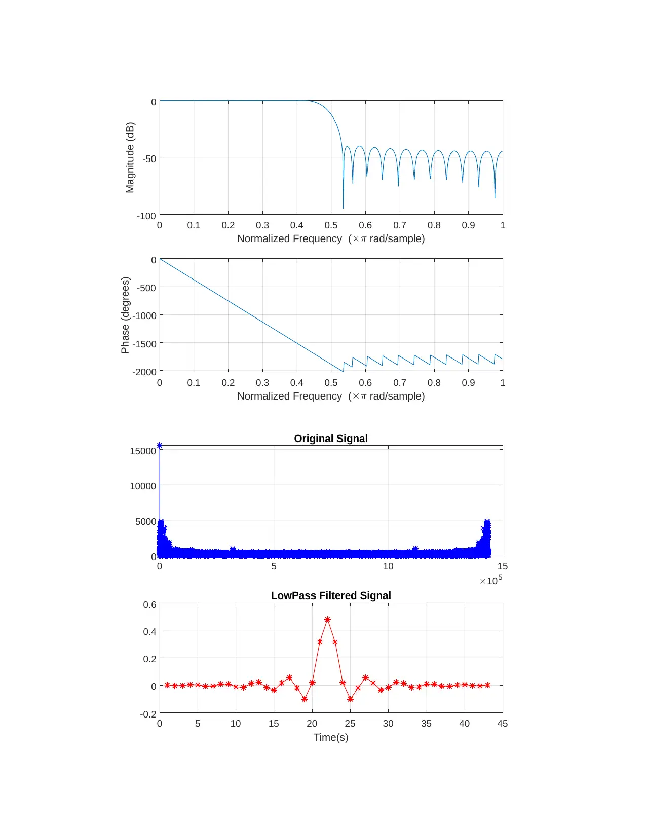
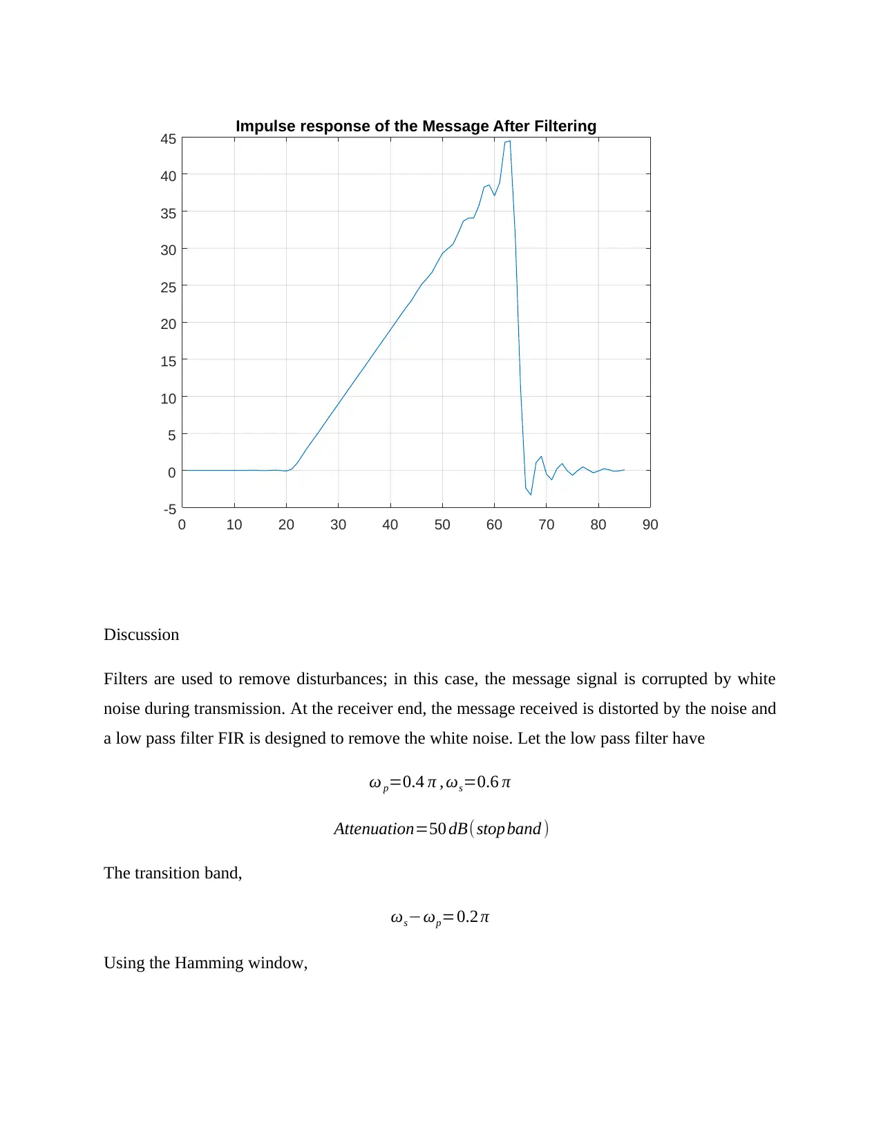
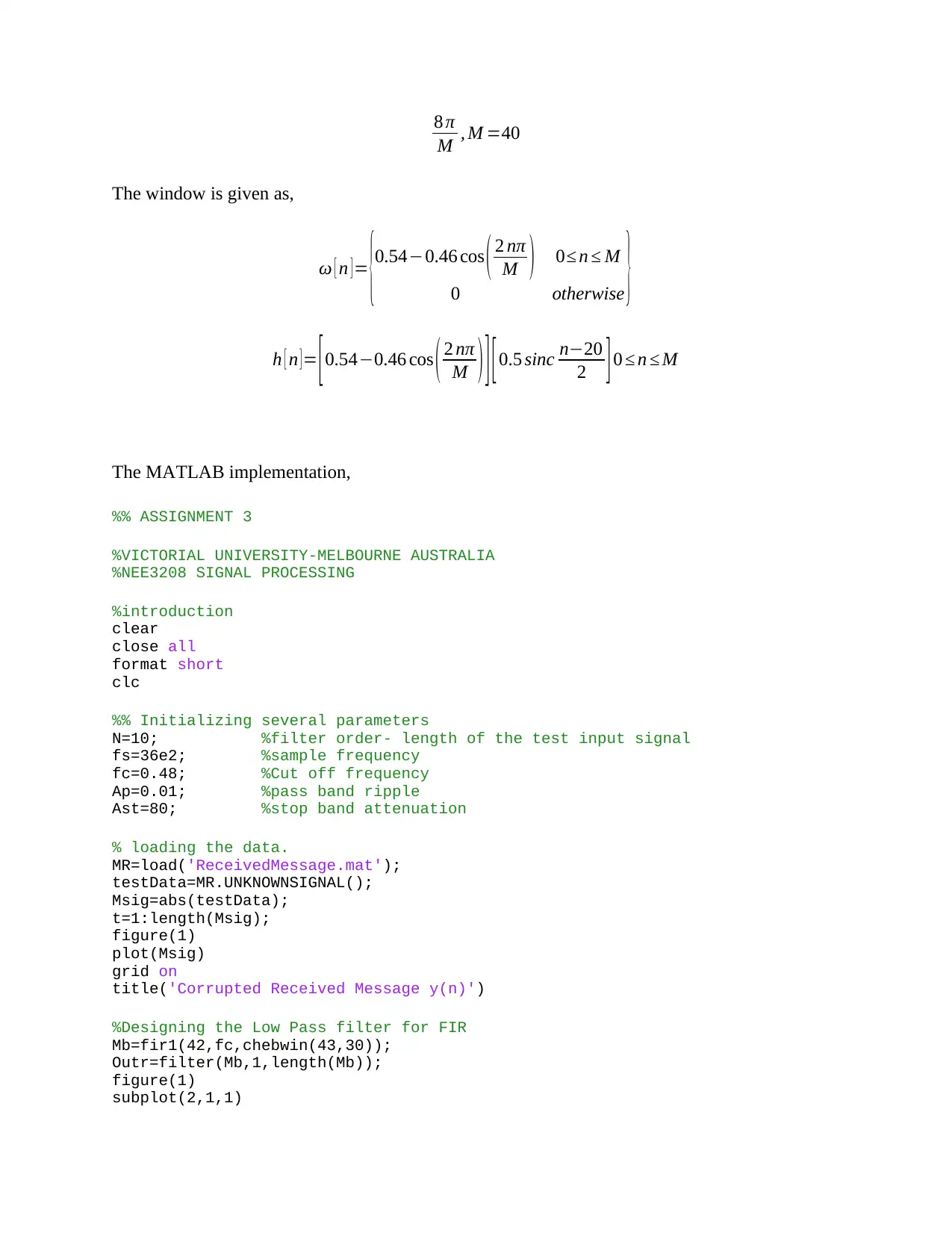
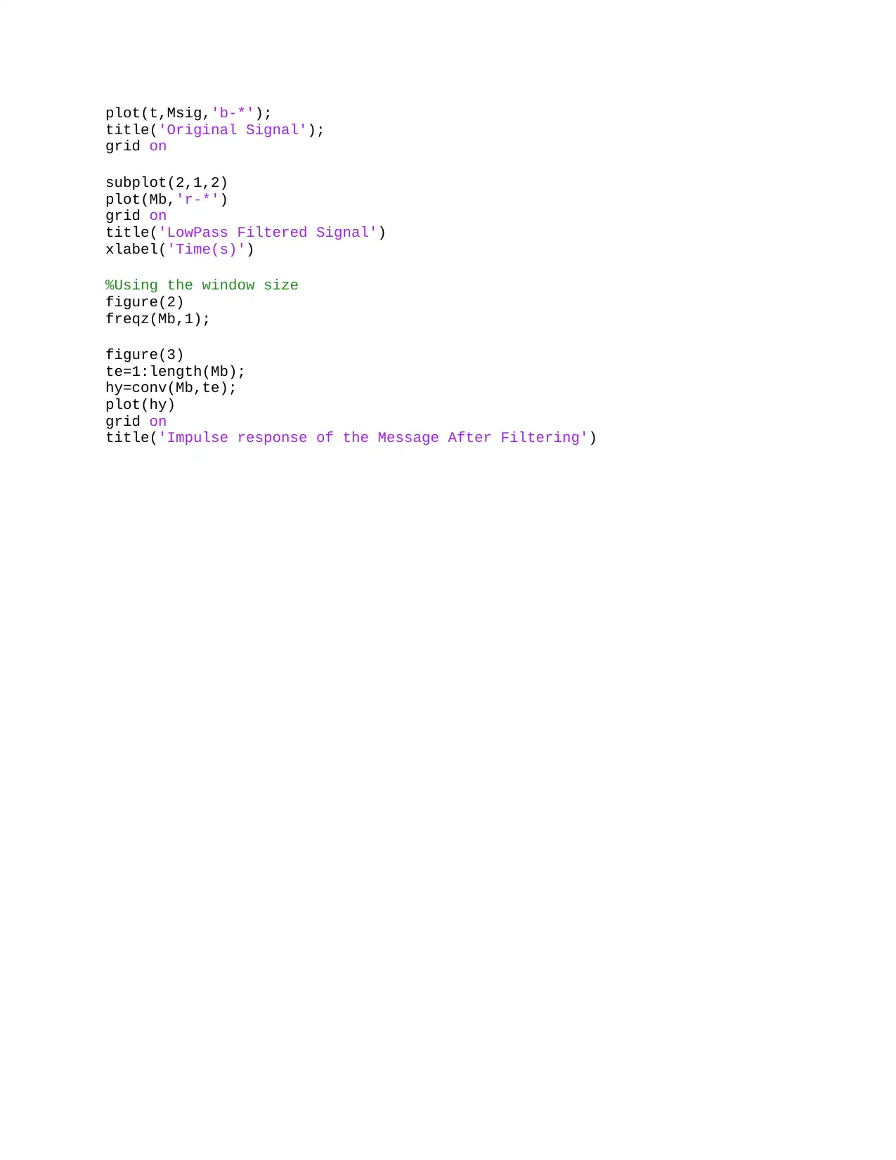
This assignment solution details the design and implementation of a Finite Impulse Response (FIR) filter to remove white noise from a corrupted message signal. The solution begins by outlining the theoretical background, including the derivation of the FIR filter's impulse response, considering the Hamming window to minimize spectral leakage. It then proceeds to evaluate the transfer function using the Discrete Fourier Transform (DFT) and analyzes the magnitude response. The solution further applies the filter in both the frequency and time domains to the input signal, illustrating the filtering process and the effect on the signal. The MATLAB implementation is provided, including the necessary parameters, data loading, and the creation of a low-pass filter using the fir1 function. The assignment includes plots of the original signal, the filtered signal, and the impulse response of the filter, demonstrating the effectiveness of the filter in removing noise and restoring the original signal. The solution also discusses the transition band and the window size used in the filter design.

DIGITAL SIGNAL PROCESSING
NEE3208 SIGNAL PROCESSING
ASSIGNMENT 3
STUDENT NAME
STUDENT ID NUMBER
INSTRUCTOR (PROFESSOR/TUTOR)
DATE OF SUBMISSION

TASK
Design of a low pass FIR filter to remove the white noise that has corrupted the message
received. The FIR filter is of the form,
y ( n )= ∑
i=0
M−1
h ( i ) x ( n−i )
Part 1
Designing the kernel filter h(n) by defining its impulse response.
The non-recursive finite impulse response is given as,
y ( n )=h ( 0 ) x ( n ) +h ( 1 ) x ( n−1 )+ …+h ( N ) x ( n−N )
N−order of the filter
For a finite duration, the impulse response is given as,
To obtain the ideal low pass filter,
  c
sin1
( ) sinc
2
c
c
cj n c
d
n
h n Ae d A A n
n
 

  


  


 
    
 


For windowing,
hw ( n ) =hd ( n ) w ( n )
¿ 1
2 π Hd ( ω )∗W ( ω )
The impulse response of the FIR filter, following the Hamming window, is, therefore, given as,
h [n]= sin ( ωc ( n−L ) )
π ( n−L ) w [ n ]
Part 2
Evaluate the transfer function using DFT. Magnitude of the transfer functions.
Hd ( ω )=DTFT {hd ( n ) }= ∑
n=−∞
+ ∞
hd ( n ) e− jωn
Part iii
Apply the filter in the frequency domain to X(k). Obtaining the inverse DFT to get filtered signal
and determining the cut-off frequency
hd ( n )=IDTFT { Hd ( ω ) }
¿ 1
2 π 
−ωc
+ωc
A e− jωn dω
¿ A ( sin ( ωc n )
πn )
¿ A ( ωc
π )sinc ( ωc
π n )
Part iv
Applying the filter in the time domain to obtain the filtered signal y(n)

0 0.1 0.2 0.3 0.4 0.5 0.6 0.7 0.8 0.9 1
Normalized Frequency ( rad/sample)
-2000
-1500
-1000
-500
0
Phase (degrees)
0 0.1 0.2 0.3 0.4 0.5 0.6 0.7 0.8 0.9 1
Normalized Frequency ( rad/sample)
-100
-50
0
Magnitude (dB)
0 5 10 15
105
0
5000
10000
15000
Original Signal
0 5 10 15 20 25 30 35 40 45
Time(s)
-0.2
0
0.2
0.4
0.6 LowPass Filtered Signal

0 10 20 30 40 50 60 70 80 90
-5
0
5
10
15
20
25
30
35
40
45 Impulse response of the Message After Filtering
Discussion
Filters are used to remove disturbances; in this case, the message signal is corrupted by white
noise during transmission. At the receiver end, the message received is distorted by the noise and
a low pass filter FIR is designed to remove the white noise. Let the low pass filter have
ω p=0.4 π , ωs=0.6 π
Attenuation=50 dB(stopband )
The transition band,
ωs−ωp=0.2 π
Using the Hamming window,

8 π
M , M =40
The window is given as,
ω [ n ] = {0.54−0.46 cos ( 2 nπ
M ) 0≤ n ≤ M
0 otherwise }
h [ n ] = [ 0.54−0.46 cos ( 2 nπ
M ) ] [ 0.5 sinc n−20
2 ] 0 ≤ n ≤ M
The MATLAB implementation,
%% ASSIGNMENT 3
%VICTORIAL UNIVERSITY-MELBOURNE AUSTRALIA
%NEE3208 SIGNAL PROCESSING
%introduction
clear
close all
format short
clc
%% Initializing several parameters
N=10; %filter order- length of the test input signal
fs=36e2; %sample frequency
fc=0.48; %Cut off frequency
Ap=0.01; %pass band ripple
Ast=80; %stop band attenuation
% loading the data.
MR=load('ReceivedMessage.mat');
testData=MR.UNKNOWNSIGNAL();
Msig=abs(testData);
t=1:length(Msig);
figure(1)
plot(Msig)
grid on
title('Corrupted Received Message y(n)')
%Designing the Low Pass filter for FIR
Mb=fir1(42,fc,chebwin(43,30));
Outr=filter(Mb,1,length(Mb));
figure(1)
subplot(2,1,1)

plot(t,Msig,'b-*');
title('Original Signal');
grid on
subplot(2,1,2)
plot(Mb,'r-*')
grid on
title('LowPass Filtered Signal')
xlabel('Time(s)')
%Using the window size
figure(2)
freqz(Mb,1);
figure(3)
te=1:length(Mb);
hy=conv(Mb,te);
plot(hy)
grid on
title('Impulse response of the Message After Filtering')