Design Project: Flood Analysis of Inverbrackie Creek (C&ENVENG 3077)
VerifiedAdded on 2022/09/08
|28
|7283
|13
Project
AI Summary
This project analyzes the flood frequency of Inverbrackie Creek, a small rural catchment near Adelaide, South Australia. It begins with an overview of the hydrological characteristics, examining seasonal variations in rainfall and runoff, and inter-annual variability. The project addresses missing data in the annual peak flow series and employs strategies like regression analysis to minimize its impact. Flood frequency analysis is performed using Gumbel and Log-normal distributions, and the results are compared. Further analysis includes FLIKE, Log-Pearson Type 3, regional frequency estimation, and the probabilistic rational method. Advanced procedures like Generalized Extreme Value and Pareto distributions are applied to refine the model, and the impacts of these methods on design flow estimates are discussed. The report concludes with a results evaluation, comparing the different techniques and their suitability for the application.
Contents
Table of figures................................................................................................................................................2
1.Overview of the Hydrological Characteristics...............................................................................................3
Seasonal Variation of Rainfall......................................................................................................................3
Seasonal Variation of Runoff.......................................................................................................................4
Inter-Annual Variation of Runoff.................................................................................................................4
Key Trends from Hydrological Characteristics............................................................................................5
2. Examine the Annual Series of Peak Flows from the Daily Flow Data.........................................................6
Identification of Missing Data......................................................................................................................6
Strategy to Minimize the Impact of Missing Data........................................................................................6
The plot of Annual Time Series of Peak Flows............................................................................................7
LOG-NORMAL PROBABILITY DISTRIBUTION....................................................................................8
3. ANALYSIS USING FLIKE.........................................................................................................................9
Flood frequency analysis using the Gumbel scale........................................................................................9
Flood frequency analysis using Log-normal distribution............................................................................13
Table of Design Flows for AEP..................................................................................................................14
4. FLOOD FREQUENCY ANALYSIS USING FLIKE- LOG-PEARSON TYPE 3.....................................14
LP-3 Probability Model..............................................................................................................................14
Probability Plot...........................................................................................................................................15
Table of Design Flows for AEP..................................................................................................................15
5. REGIONAL FREQUENCY ESTIMATION..............................................................................................16
Key Inputs..................................................................................................................................................16
Key Differences in the Estimation of Flows...............................................................................................18
6. Probabilistic Rational method.....................................................................................................................18
7. ADVANCED PROCEDURES IN FLIKE..................................................................................................21
Generalized Extreme Value Function.........................................................................................................21
Pareto Distribution.....................................................................................................................................21
Comparison of Probability Plots.................................................................................................................22
Impacts of Advanced methods on Model Fit..............................................................................................22
Design Flow Estimates of advanced methods for AEP...............................................................................23
Impacts of advanced methods to Design flow-Reasons..............................................................................23
RESULTS EVALUATION............................................................................................................................23
Potential Reasons for Differences in the Model fitting...............................................................................24
References......................................................................................................................................................25
Paraphrase This Document
Need a fresh take? Get an instant paraphrase of this document with our AI Paraphraser
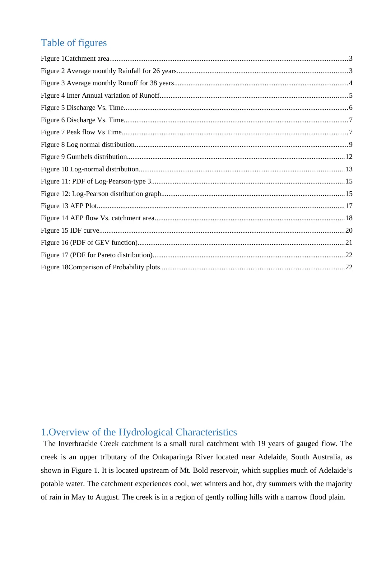
Table of figures
Figure 1Catchment area....................................................................................................................................3
Figure 2 Average monthly Rainfall for 26 years..............................................................................................3
Figure 3 Average monthly Runoff for 38 years................................................................................................4
Figure 4 Inter Annual variation of Runoff........................................................................................................5
Figure 5 Discharge Vs. Time............................................................................................................................6
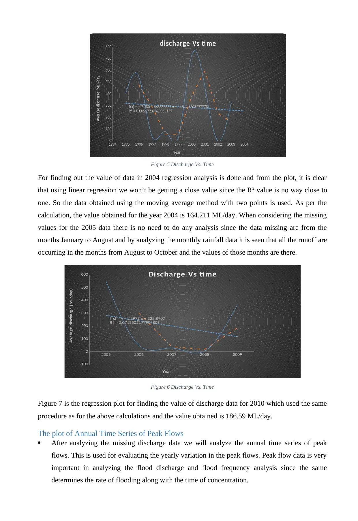
Figure 6 Discharge Vs. Time............................................................................................................................7
Figure 7 Peak flow Vs Time.............................................................................................................................7
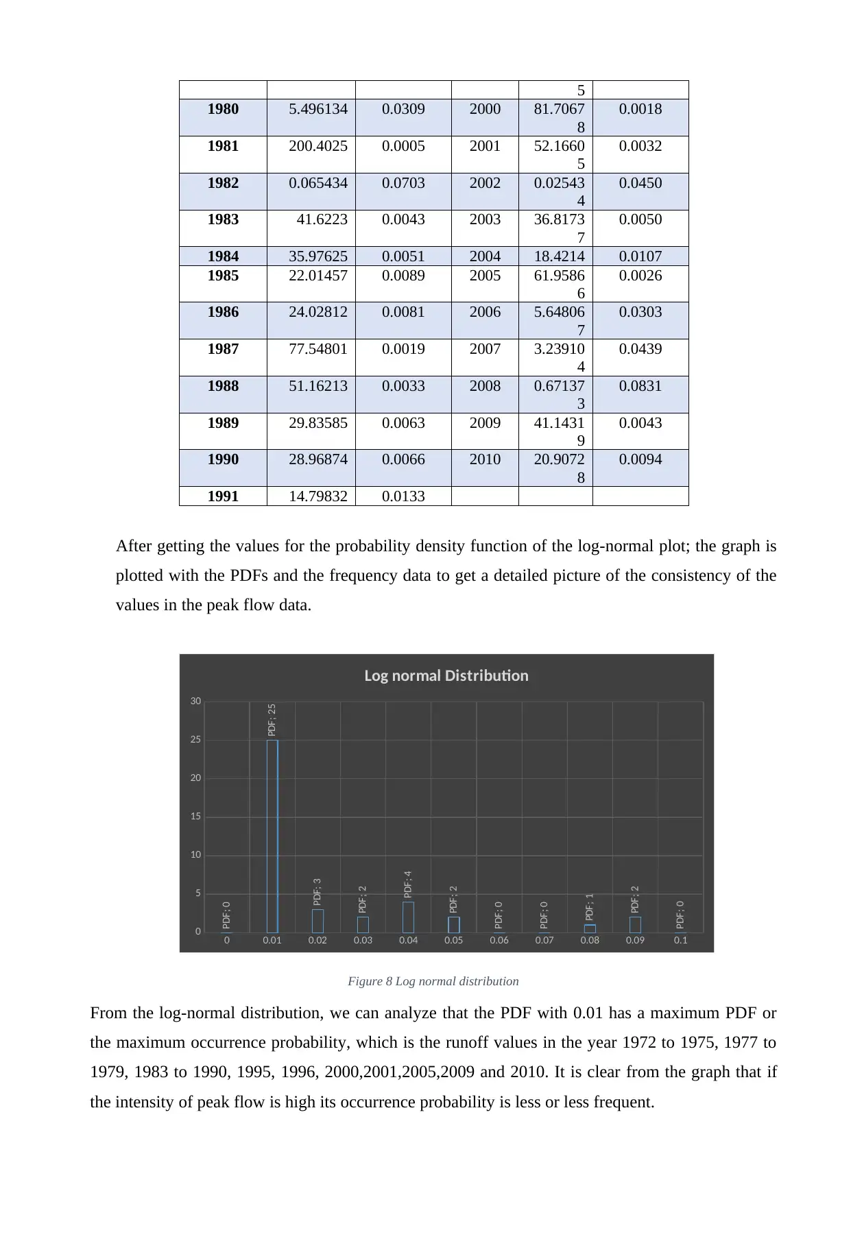
Figure 8 Log normal distribution......................................................................................................................9
Figure 9 Gumbels distribution........................................................................................................................12
Figure 10 Log-normal distribution.................................................................................................................13
Figure 11: PDF of Log-Pearson-type 3...........................................................................................................15
Figure 12: Log-Pearson distribution graph.....................................................................................................15
Figure 13 AEP Plot........................................................................................................................................17
Figure 14 AEP flow Vs. catchment area.........................................................................................................18
Figure 15 IDF curve.......................................................................................................................................20
Figure 16 (PDF of GEV function)..................................................................................................................21
Figure 17 (PDF for Pareto distribution)..........................................................................................................22
Figure 18Comparison of Probability plots......................................................................................................22
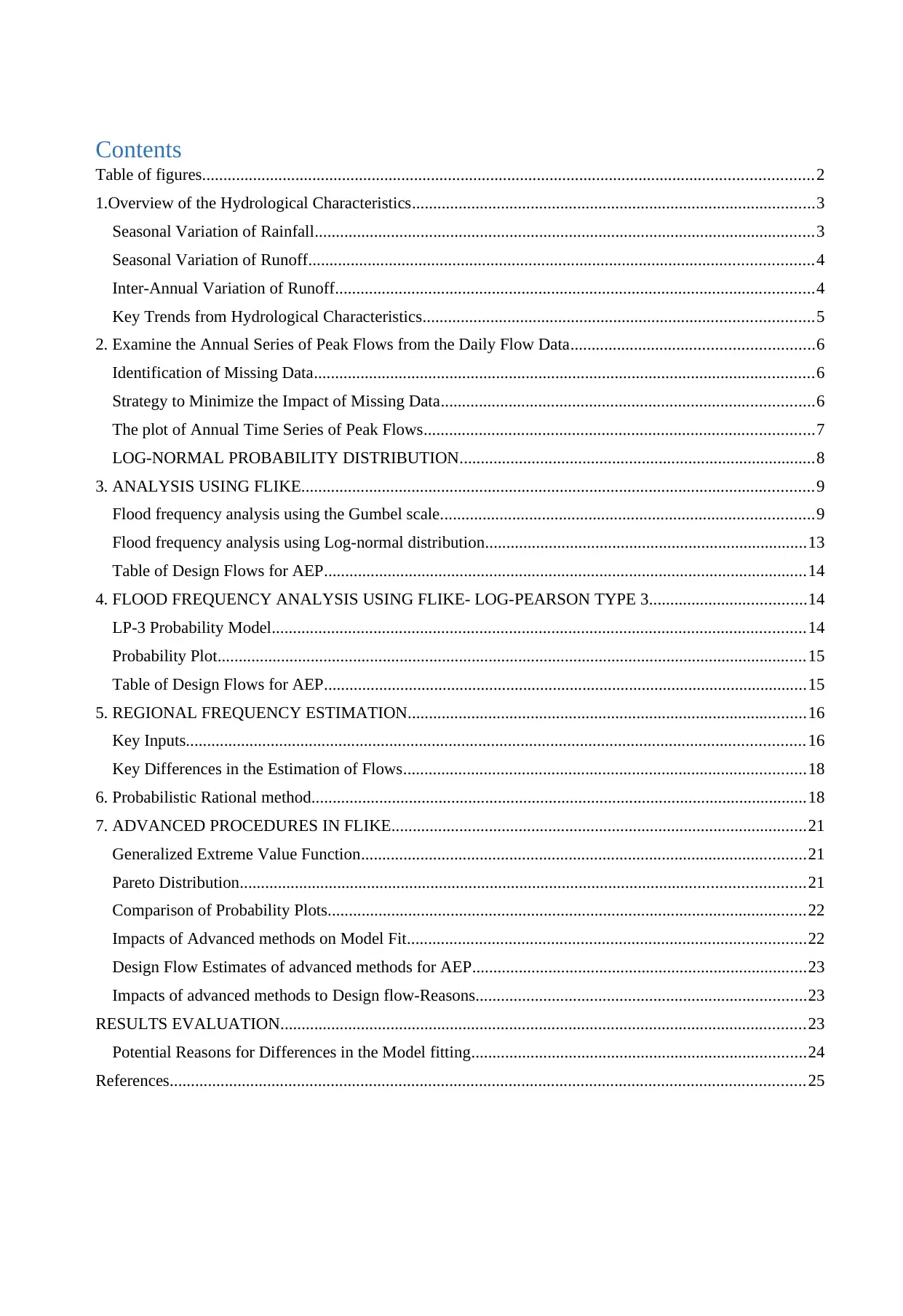
1.Overview of the Hydrological Characteristics
The Inverbrackie Creek catchment is a small rural catchment with 19 years of gauged flow. The
creek is an upper tributary of the Onkaparinga River located near Adelaide, South Australia, as
shown in Figure 1. It is located upstream of Mt. Bold reservoir, which supplies much of Adelaide’s
potable water. The catchment experiences cool, wet winters and hot, dry summers with the majority
of rain in May to August. The creek is in a region of gently rolling hills with a narrow flood plain.
Figure 1Catchment area....................................................................................................................................3
Figure 2 Average monthly Rainfall for 26 years..............................................................................................3
Figure 3 Average monthly Runoff for 38 years................................................................................................4
Figure 4 Inter Annual variation of Runoff........................................................................................................5
Figure 5 Discharge Vs. Time............................................................................................................................6
Figure 6 Discharge Vs. Time............................................................................................................................7
Figure 7 Peak flow Vs Time.............................................................................................................................7
Figure 8 Log normal distribution......................................................................................................................9
Figure 9 Gumbels distribution........................................................................................................................12
Figure 10 Log-normal distribution.................................................................................................................13
Figure 11: PDF of Log-Pearson-type 3...........................................................................................................15
Figure 12: Log-Pearson distribution graph.....................................................................................................15
Figure 13 AEP Plot........................................................................................................................................17
Figure 14 AEP flow Vs. catchment area.........................................................................................................18
Figure 15 IDF curve.......................................................................................................................................20
Figure 16 (PDF of GEV function)..................................................................................................................21
Figure 17 (PDF for Pareto distribution)..........................................................................................................22
Figure 18Comparison of Probability plots......................................................................................................22
1.Overview of the Hydrological Characteristics
The Inverbrackie Creek catchment is a small rural catchment with 19 years of gauged flow. The
creek is an upper tributary of the Onkaparinga River located near Adelaide, South Australia, as
shown in Figure 1. It is located upstream of Mt. Bold reservoir, which supplies much of Adelaide’s
potable water. The catchment experiences cool, wet winters and hot, dry summers with the majority
of rain in May to August. The creek is in a region of gently rolling hills with a narrow flood plain.
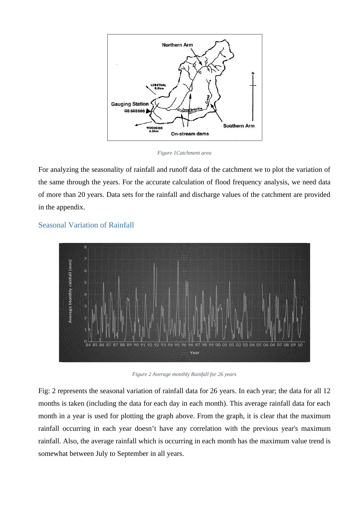
Figure 1Catchment area
For analyzing the seasonality of rainfall and runoff data of the catchment we to plot the variation of
the same through the years. For the accurate calculation of flood frequency analysis, we need data
of more than 20 years. Data sets for the rainfall and discharge values of the catchment are provided
in the appendix.
Seasonal Variation of Rainfall
84 85 86 87 87 88 89 90 91 92 92 93 94 95 96 96 97 98 99 00 01 01 02 03 04 05 06 06 07 08 09 10
0
1
2
3
4
5
6
7
8
Year
Average Monthly rainfall (mm)
Figure 2 Average monthly Rainfall for 26 years
Fig: 2 represents the seasonal variation of rainfall data for 26 years. In each year; the data for all 12
months is taken (including the data for each day in each month). This average rainfall data for each
month in a year is used for plotting the graph above. From the graph, it is clear that the maximum
rainfall occurring in each year doesn’t have any correlation with the previous year's maximum
rainfall. Also, the average rainfall which is occurring in each month has the maximum value trend is
somewhat between July to September in all years.
⊘ This is a preview!⊘
Do you want full access?
Subscribe today to unlock all pages.
Trusted by 1+ million students worldwide
Seasonal Variation of Runoff
72
73
75
77
78
80
82
83
85
87
88
90
92
93
95
96
98
00
01
03
05
06
08
100
0.5
1
1.5
2
2.5
3
3.5
4
4.5
Years
Average Runoff (mm)
Figure 3 Average monthly Runoff for 38 years
Figure 3 represents the average runoff (mm) of the catchment for 38 years. Average discharge data
for each day for each month in a year is taken for finding the value of runoff. For getting the value
of runoff the discharge data is divided by the area of the catchment. The graph is obtained by
plotting the data for each month for 38 years. From the graph, it is clear that for every year the
average value of runoff is not showing a close correlation. This can be seen from the data of 1994,
where the value of discharge shows drastic variation from the preceding and succeeding years. So
we cannot straight away come up with a relation in the trends of runoff data Inter-annual variability
rainfall and runoff data
Inter-Annual Variation of Runoff
1972
1973
1974
1975
1976
1977
1978
1979
1980
1981
1982
1983
1984
1985
1986
1987
1988
1989
1990
1991
1992
1993
1994
1995
1996
1997
1998
1999
2000
2001
2002
2003
2004
2005
2006
2007
2008
2009
2010
0
0.2
0.4
0.6
0.8
1
1.2
Inter-annaual variation of Runoff
Year
Runoff (mm)
Figure 4 Inter Annual variation of Runoff
Key Trends from Hydrological Characteristics
Interannual variability of annual rainfall data is required to analyses the yearly variation of rainfall
and runoff. This will give a clear cut picture of the trend in the rainfall and the runoff pattern. This
is also required for the assumptions and provides a basis for further analysis.
Paraphrase This Document
Need a fresh take? Get an instant paraphrase of this document with our AI Paraphraser
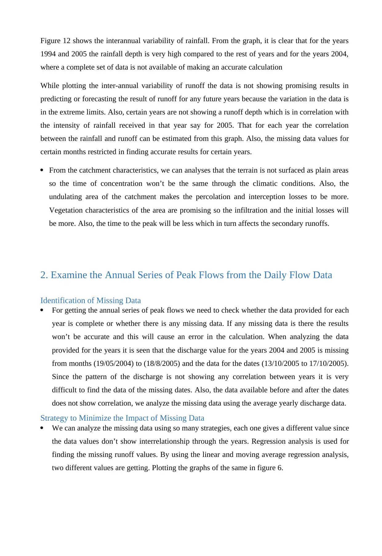
Figure 12 shows the interannual variability of rainfall. From the graph, it is clear that for the years
1994 and 2005 the rainfall depth is very high compared to the rest of years and for the years 2004,
where a complete set of data is not available of making an accurate calculation
While plotting the inter-annual variability of runoff the data is not showing promising results in
predicting or forecasting the result of runoff for any future years because the variation in the data is
in the extreme limits. Also, certain years are not showing a runoff depth which is in correlation with
the intensity of rainfall received in that year say for 2005. That for each year the correlation
between the rainfall and runoff can be estimated from this graph. Also, the missing data values for
certain months restricted in finding accurate results for certain years.
From the catchment characteristics, we can analyses that the terrain is not surfaced as plain areas
so the time of concentration won’t be the same through the climatic conditions. Also, the
undulating area of the catchment makes the percolation and interception losses to be more.
Vegetation characteristics of the area are promising so the infiltration and the initial losses will
be more. Also, the time to the peak will be less which in turn affects the secondary runoffs.
2. Examine the Annual Series of Peak Flows from the Daily Flow Data
Identification of Missing Data
For getting the annual series of peak flows we need to check whether the data provided for each
year is complete or whether there is any missing data. If any missing data is there the results
won’t be accurate and this will cause an error in the calculation. When analyzing the data
provided for the years it is seen that the discharge value for the years 2004 and 2005 is missing
from months (19/05/2004) to (18/8/2005) and the data for the dates (13/10/2005 to 17/10/2005).
Since the pattern of the discharge is not showing any correlation between years it is very
difficult to find the data of the missing dates. Also, the data available before and after the dates
does not show correlation, we analyze the missing data using the average yearly discharge data.
Strategy to Minimize the Impact of Missing Data
We can analyze the missing data using so many strategies, each one gives a different value since
the data values don’t show interrelationship through the years. Regression analysis is used for
finding the missing runoff values. By using the linear and moving average regression analysis,
two different values are getting. Plotting the graphs of the same in figure 6.
1994 1995 1996 1997 1998 1999 2000 2001 2002 2003 2004
0
100
200
300
400
500
600
700
800
f(x) = − 7.28011666666667 x + 14844.8303277778
R² = 0.00567237879365157
discharge Vs time
Year
Average discharge (ML)/day
Figure 5 Discharge Vs. Time
For finding out the value of data in 2004 regression analysis is done and from the plot, it is clear
that using linear regression we won’t be getting a close value since the R2 value is no way close to
one. So the data obtained using the moving average method with two points is used. As per the
calculation, the value obtained for the year 2004 is 164.211 ML/day. When considering the missing
values for the 2005 data there is no need to do any analysis since the data missing are from the
months January to August and by analyzing the monthly rainfall data it is seen that all the runoff are
occurring in the months from August to October and the values of those months are there.
2005 2006 2007 2008 2009
-100
0
100
200
300
400
500
600
f(x) = − 41.5973 x + 325.8907
R² = 0.0715502177904803
Discharge Vs ti me
Year
Average discharge (ML/day)
Figure 6 Discharge Vs. Time
Figure 7 is the regression plot for finding the value of discharge data for 2010 which used the same
procedure as for the above calculations and the value obtained is 186.59 ML/day.
The plot of Annual Time Series of Peak Flows
After analyzing the missing discharge data we will analyze the annual time series of peak
flows. This is used for evaluating the yearly variation in the peak flows. Peak flow data is very
important in analyzing the flood discharge and flood frequency analysis since the same
determines the rate of flooding along with the time of concentration.
0
100
200
300
400
500
600
700
800
f(x) = − 7.28011666666667 x + 14844.8303277778
R² = 0.00567237879365157
discharge Vs time
Year
Average discharge (ML)/day
Figure 5 Discharge Vs. Time
For finding out the value of data in 2004 regression analysis is done and from the plot, it is clear
that using linear regression we won’t be getting a close value since the R2 value is no way close to
one. So the data obtained using the moving average method with two points is used. As per the
calculation, the value obtained for the year 2004 is 164.211 ML/day. When considering the missing
values for the 2005 data there is no need to do any analysis since the data missing are from the
months January to August and by analyzing the monthly rainfall data it is seen that all the runoff are
occurring in the months from August to October and the values of those months are there.
2005 2006 2007 2008 2009
-100
0
100
200
300
400
500
600
f(x) = − 41.5973 x + 325.8907
R² = 0.0715502177904803
Discharge Vs ti me
Year
Average discharge (ML/day)
Figure 6 Discharge Vs. Time
Figure 7 is the regression plot for finding the value of discharge data for 2010 which used the same
procedure as for the above calculations and the value obtained is 186.59 ML/day.
The plot of Annual Time Series of Peak Flows
After analyzing the missing discharge data we will analyze the annual time series of peak
flows. This is used for evaluating the yearly variation in the peak flows. Peak flow data is very
important in analyzing the flood discharge and flood frequency analysis since the same
determines the rate of flooding along with the time of concentration.
⊘ This is a preview!⊘
Do you want full access?
Subscribe today to unlock all pages.
Trusted by 1+ million students worldwide
1972
1973
1974
1975
1976
1977
1978
1979
1980
1981
1982
1983
1984
1985
1986
1987
1988
1989
1990
1991
1992
1993
1994
1995
1996
1997
1998
1999
2000
2001
2002
2003
2004
2005
2006
2007
2008
2009
20100
50
100
150
200
250
Peak fl ow Vs ti me
Year
Runoff (mm)
Figure 7 Peak flow Vs Time
Figure 8 represents the peak flow of runoff through years including the missing data. From the
graph, we can see that peak flow occurred with a maximum value exceeding 150 mm/day only for
two years that is 1981 and 1992. The rest of the years shows almost the same range in the peak
flow. Analyzing this we will get an awareness about the return period of the flood which is likely to
occur. Since the data is not showing a close likely hood of a relationship, relying on a single method
of analysis of flood frequency won’t be sufficient.
LOG-NORMAL PROBABILITY DISTRIBUTION
By creating a log-normal probability distribution for the annual peak flows help to get an idea
about the frequency in the occurrence of the peak flows of the range of data.
Year Runoff Log-
Normal
Distributio
n
Year Runoff Log-
Normal
Distributio
n
1972 38.66476 0.0047 1992 175.416
5
0.0006
1973 71.93109 0.0021 1993 6.95529
4
0.0258
1974 56.47888 0.0029 1994 0.14565
8
0.0865
1975 92.92964 0.0015 1995 45.2866
1
0.0039
1976 16.52908 0.0119 1996 61.1961
9
0.0026
1977 72.01927 0.0021 1997 4.26151
3
0.0369
1978 60.01815 0.0027 1998 9.06857
1
0.0208
1979 43.22958 0.0041 1999 3.80134 0.0397
Paraphrase This Document
Need a fresh take? Get an instant paraphrase of this document with our AI Paraphraser
5
1980 5.496134 0.0309 2000 81.7067
8
0.0018
1981 200.4025 0.0005 2001 52.1660
5
0.0032
1982 0.065434 0.0703 2002 0.02543
4
0.0450
1983 41.6223 0.0043 2003 36.8173
7
0.0050
1984 35.97625 0.0051 2004 18.4214 0.0107
1985 22.01457 0.0089 2005 61.9586
6
0.0026
1986 24.02812 0.0081 2006 5.64806
7
0.0303
1987 77.54801 0.0019 2007 3.23910
4
0.0439
1988 51.16213 0.0033 2008 0.67137
3
0.0831
1989 29.83585 0.0063 2009 41.1431
9
0.0043
1990 28.96874 0.0066 2010 20.9072
8
0.0094
1991 14.79832 0.0133
After getting the values for the probability density function of the log-normal plot; the graph is
plotted with the PDFs and the frequency data to get a detailed picture of the consistency of the
values in the peak flow data.
0 0.01 0.02 0.03 0.04 0.05 0.06 0.07 0.08 0.09 0.1
0
5
10
15
20
25
30
PDF; 0
PDF; 25
PDF; 3
PDF; 2
PDF; 4
PDF; 2
PDF; 0
PDF; 0
PDF; 1
PDF; 2
PDF; 0
Log normal Distribution
Figure 8 Log normal distribution
From the log-normal distribution, we can analyze that the PDF with 0.01 has a maximum PDF or
the maximum occurrence probability, which is the runoff values in the year 1972 to 1975, 1977 to
1979, 1983 to 1990, 1995, 1996, 2000,2001,2005,2009 and 2010. It is clear from the graph that if
the intensity of peak flow is high its occurrence probability is less or less frequent.
3. ANALYSIS USING FLIKE
Flood frequency analysis using the Gumbel scale.
For finding out the value of expected outcomes of design peak flows and for doing the flood
frequency analysis several methods has to be applied and the best of the fitting data is used for the
analysis. In Gumbel’s Type 1 distribution first, we need to identify the Probability of occurrence of
an event and its associated return period. For finding the probability (p) (%) we are using the
Weibull's formula which is p= m/ (N+1), where m is the rank of the events when the events are
arranged in the ascending order an N is the total number of data. After finding the value of p, the
return period of floods is calculated which is the reciprocal of probability. The tabular format of
finding the estimated return period is given below.
Yea
r
Max
discharg
e
(m3/sec)
Ran
k
(m)
P %
m/(N+1
)
T
estimated
=1/(p)
Yea
r
Max
discharge
(m3/sec)
Rank
(m)
P %
m/(N+1
)
T
estimate
d =1/(p)
1981 20.70129
6
1 0.025 40.0 1989 3.0820023
1
21 0.525 1.9
1992 18.12027
8
2 0.05 20.0 1990 2.9924305
6
22 0.55 1.8
1975 9.599502
3
3 0.075 13.3 1986 2.4820717
6
23 0.575 1.7
2000 8.440196
8
4 0.1 10.0 1985 2.2740740
7
24 0.6 1.7
1987 8.010601
9
5 0.125 8.0 2010 2.1596932
9
25 0.625 1.6
1977 7.439490
7
6 0.15 6.7 2004 1.9029050
9
26 0.65 1.5
1973 7.430381
9
7 0.175 5.7 1976 1.7074305
6
27 0.675 1.5
2005 6.400243
1
8 0.2 5.0 1991 1.5286458
3
28 0.7 1.4
1996 6.321481
5
9 0.225 4.4 1998 0.9367708
3
29 0.725 1.4
1978 6.199791
7
10 0.25 4.0 1993 0.7184722
2
30 0.75 1.3
1974 5.834189
8
11 0.275 3.6 2006 0.5834375 31 0.775 1.3
2001 5.388680
6
12 0.3 3.3 1980 0.5677430
6
32 0.8 1.3
1988 5.284976
9
13 0.325 3.1 1997 0.4402083
3
33 0.825 1.2
1995 4.678044 14 0.35 2.9 1999 0.3926736
1
34 0.85 1.2
1979 4.465555
6
15 0.375 2.7 2007 0.3345949
1
35 0.875 1.1
1983 4.299525
5
16 0.4 2.5 2008 0.0693518
5
36 0.9 1.1
2009 4.250034
7
17 0.425 2.4 1994 0.0150463 37 0.925 1.1
1972 3.994016 18 0.45 2.2 1982 0.0067592 38 0.95 1.1
⊘ This is a preview!⊘
Do you want full access?
Subscribe today to unlock all pages.
Trusted by 1+ million students worldwide
2 6
2003 3.803182
9
19 0.475 2.1 2002 0.0026273
1
39 0.975 1.0
1984 3.716296
3
20 0.5 2.0
After finding the estimated value of T, for analyzing the theoretical value and to find the flood
frequency analysis we need to find the theoretical value of T. For that we are using the equation,
Where x= observed peak flow data
u = x – 0.5772 α
α= ¿ ×Sx)/ π
x = Mean of x and Sx = Standard deviation of x
So the value, Average x = 4.271146278
Standard deviation Sx =4.479047066
α= ¿ ×4.479047066)/ π = 3.49229
u = 4.271146278 – (0.5772 ×3.49229) = 2.2535
Year
Max
discharg
e
(m3/sec)
(x-u)/α p T
T
theoretic
al
Yea
r
Max
discharg
e
(ML/day
)
Max
discharg
e
(m3/sec)
(x-
u)/α p T
T
theoretic
al
1981 20.7012 5.2824 0.0 197.342 1989 266.285 3.082002 0.237 0.5 1.832777
1992 18.1202 4.5433 0.0 94.5051 1990 258.546 2.992431 0.211 0.6 1.802330
1975 9.59950 2.1034 0.1 8.70467 1986 214.451 2.482072 0.065 0.6 1.644554
2000 8.44019 1.7715 0.2 6.39385 1985 196.48 2.274074 0.005 0.6 1.587399
1987 8.01060 1.6484 0.2 5.715152 2010 186.5975 2.159693 -0.026 0.6 1.557610
1977 7.43949 1.4849 0.2 4.93363 2004 164.411 1.902905 -0.100 0.7 1.494775
1973 7.43038 1.4823 0.2 4.92218 1976 147.522 1.707431 -0.156 0.7 1.450518
2005 6.40024 1.1873 0.3 3.80384 1991 132.075 1.528646 -0.207 0.7 1.412607
1996 6.32148 1.1648 0.3 3.73130 1998 80.937 0.936771 -0.377 0.8 1.303276
1978 6.19979 1.1299 0.3 3.62245 1993 62.076 0.718472 -0.439 0.8 1.268739
Paraphrase This Document
Need a fresh take? Get an instant paraphrase of this document with our AI Paraphraser
1974 5.83418 1.0252 0.3 3.31772 2006 50.409 0.583438 -0.478 0.8 1.248820
2001 5.38868 0.8977 0.3 2.98786 1980 49.053 0.567743 -0.482 0.8 1.246574
1988 5.28497 0.8680 0.3 2.91707 1997 38.034 0.440208 -0.519 0.8 1.228851
1995 4.678044 0.6942 0.4 2.543622 1999 33.927 0.392674 -0.532 0.8 1.222481
1979 4.46555 0.6333 0.4 2.42800 2007 28.909 0.334595 -0.549 0.8 1.214867
1983 4.29952 0.5858 0.4 2.342659 2008 5.992 0.069352 -0.62 0.8 1.182406
2009 4.25003 0.5716 0.4 2.31803 1994 1.3 0.015046 -0.641 0.9 1.176213
1972 3.994016 0.4983 0.5 2.196346 1982 0.584 0.006759 -0.643 0.9 1.175281
2003 3.803182 0.4437 0.5 2.111603 2002 0.227 0.002627 -0.644 0.9 1.174818
1984 3.716296 0.4188 0.5 2.074625
Thus we got the values for the theoretical value of the return period. Plot the probability plot of the
flood frequency analysis to analyze the data variation concerning the theoretical using Gumbel
distribution. In the plot, the return period is plotted on a logarithmic scale to get a clear cut picture
of the variation in the same with the annual peak flow data. Here, the scattered smooth line in
orange color represents the theoretical distribution and the scatter plot with blue dots represents the
fit of the annual peak flow data concerning a Gumbel distribution. Using this plot, we can predict
the flow values of the stream corresponding to any return period from 1 to 100. It should be noted
that the curve follows the distribution in a perfect fit for low flows but slides away from the
theoretical distribution at higher values of flows. So, this is the reason that we are forced to use
multiple distributions such as log-normal or log Pearson type III and to check the perfect fitting data
set for a particular site.
0.2 2.0 20.0 200.0
0
5
10
15
20
25
Gumbel's distributi on
T-estimated T-theoretical
Return period
Peak stream flow (m3/s)
Figure 9 Gumbels distribution
From the graph in figure 5, we will be able to predict the annual exceedance probability design
flows concerning any return periods, which should be compared with the theoretical AEP which is
been found out from Gumbel’s type 1 distribution by equations. For finding the flood discharge
with a recurrence in 100 years we will be using the equation; XT= x + (KT ×Sx)
Where XT = Value of design flood with return period T years
x = Man of the observed values
KT = modified frequency factor = (yT- yn) Sn
yn = reduced mean; whose value = 0.5430 for N= 39 (data available for analysis)
Sn= reduced standard deviation; whose value = 1.1388 for N= 39 (data available for
analysis)
YT = reduced variate = - [ln (ln (T/T-1))]
Therefore YT = - [ln (ln (100/100-1))] = 4.6001
KT = (4.6001- 0.5430)/1.1338
= 3.562
XT = 4.271146278 + (3.562×4.479047066)
= 20.22 m3/s
This is the value of peak flood discharge with a return period of once in 100 years. The same
obtained from the graph of Gumbel’s distribution of theoretical return period Vs. peak flow is 18.5
m3/s. We can see a wide variation in the result if the value is for a high return period, which is
depicting from the graph. The table below shows the values of peak streamflow data for different
return periods both from the estimated T and from the theoretical T from the method.
AEP Q theoretical Q Estimated
⊘ This is a preview!⊘
Do you want full access?
Subscribe today to unlock all pages.
Trusted by 1+ million students worldwide
1 out of 28
Related Documents


Your All-in-One AI-Powered Toolkit for Academic Success.
+13062052269
info@desklib.com
Available 24*7 on WhatsApp / Email
![[object Object]](/_next/static/media/star-bottom.7253800d.svg)
Unlock your academic potential
Copyright © 2020–2026 A2Z Services. All Rights Reserved. Developed and managed by ZUCOL.