Hydrology Report: Flood Analysis for Tillergra Dam Construction

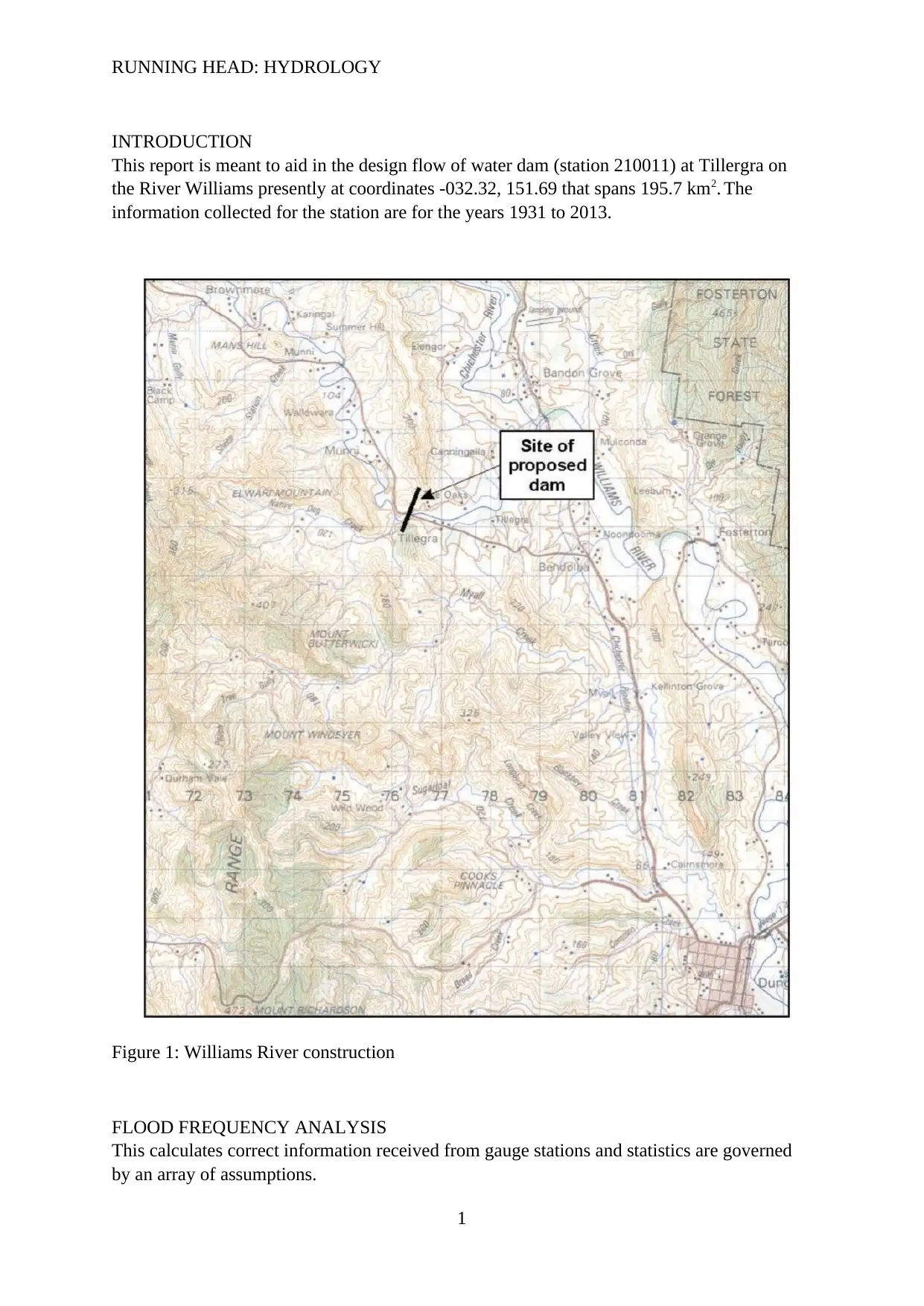
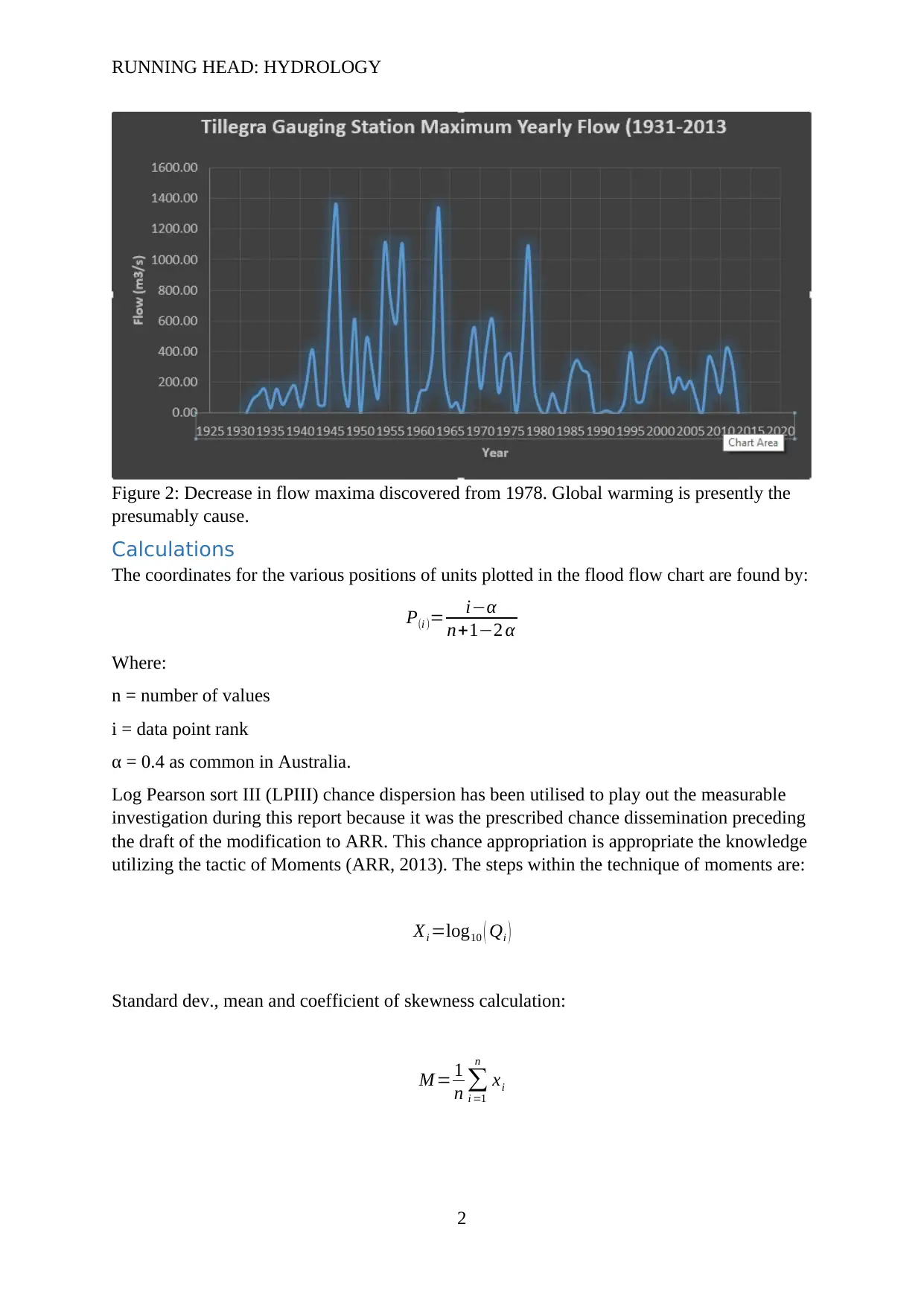
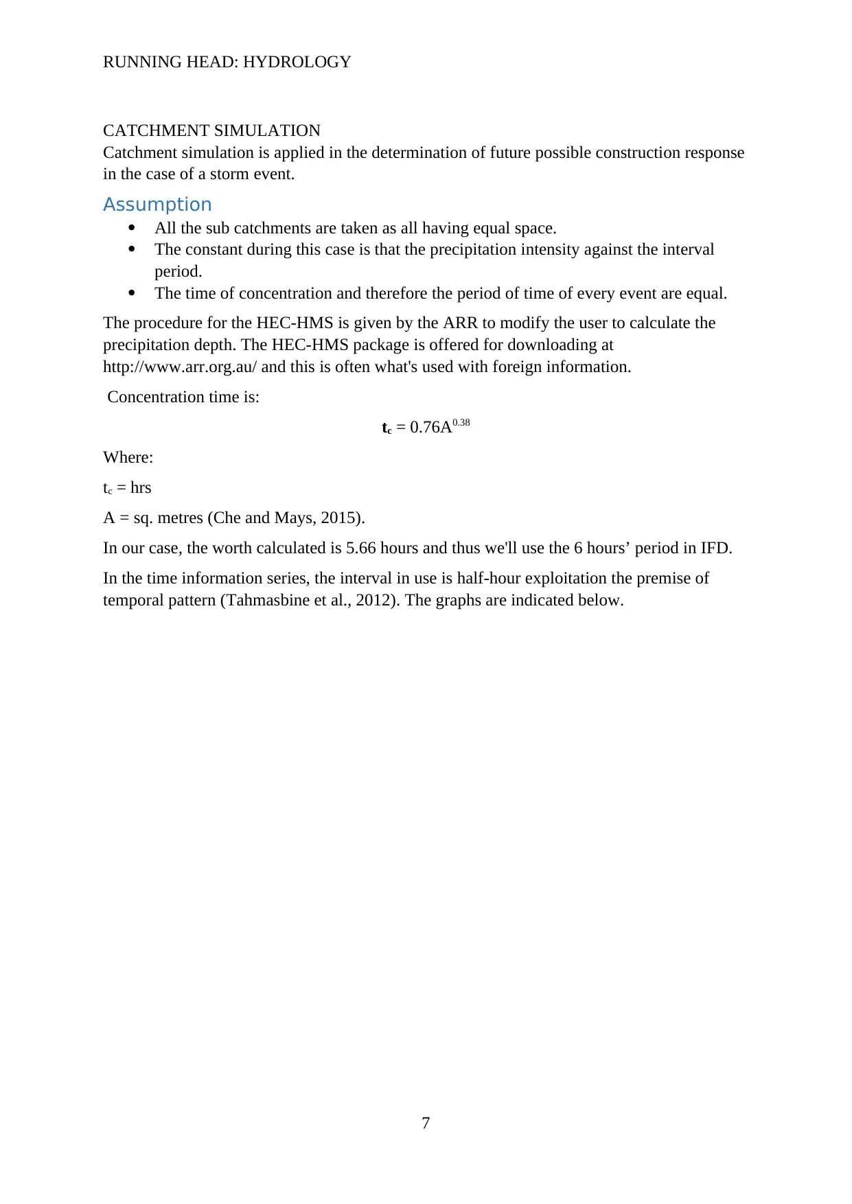
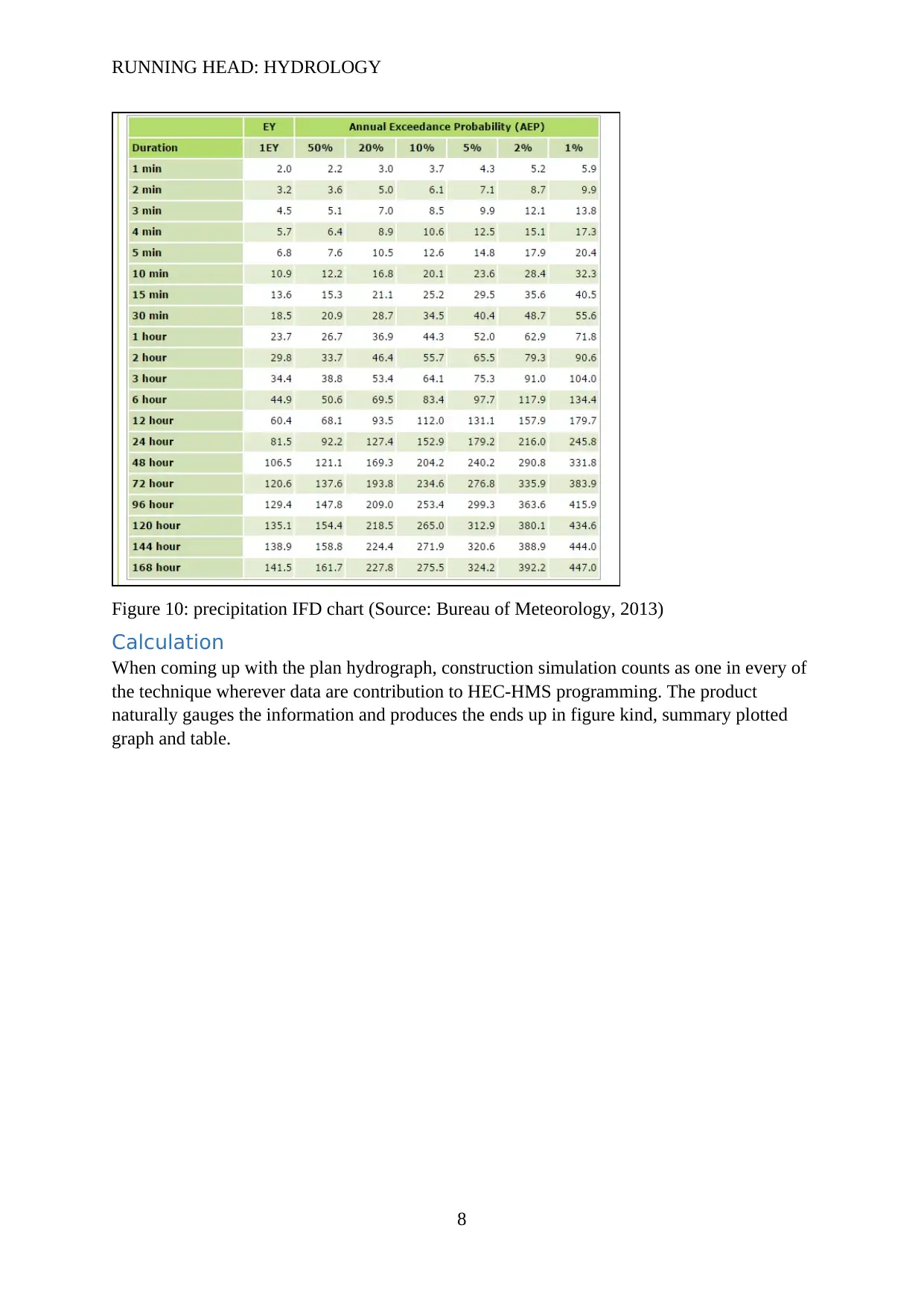
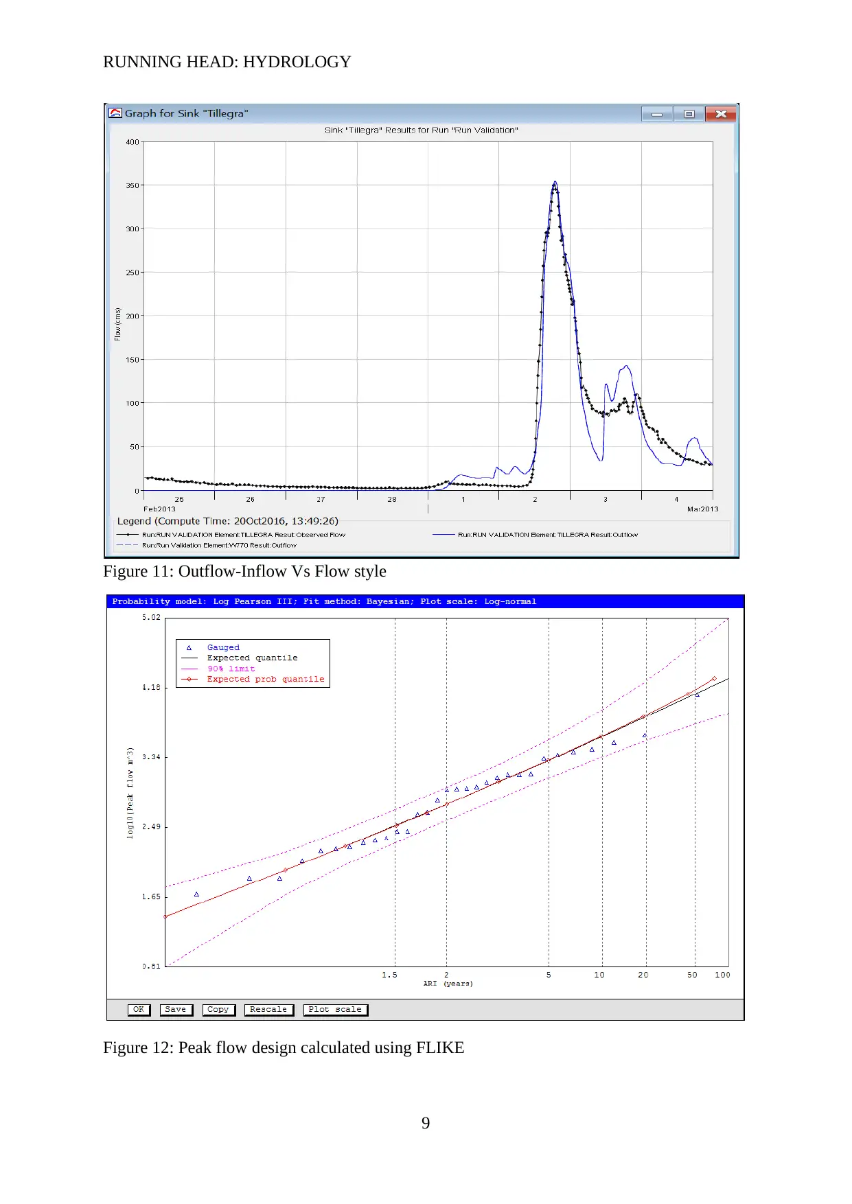
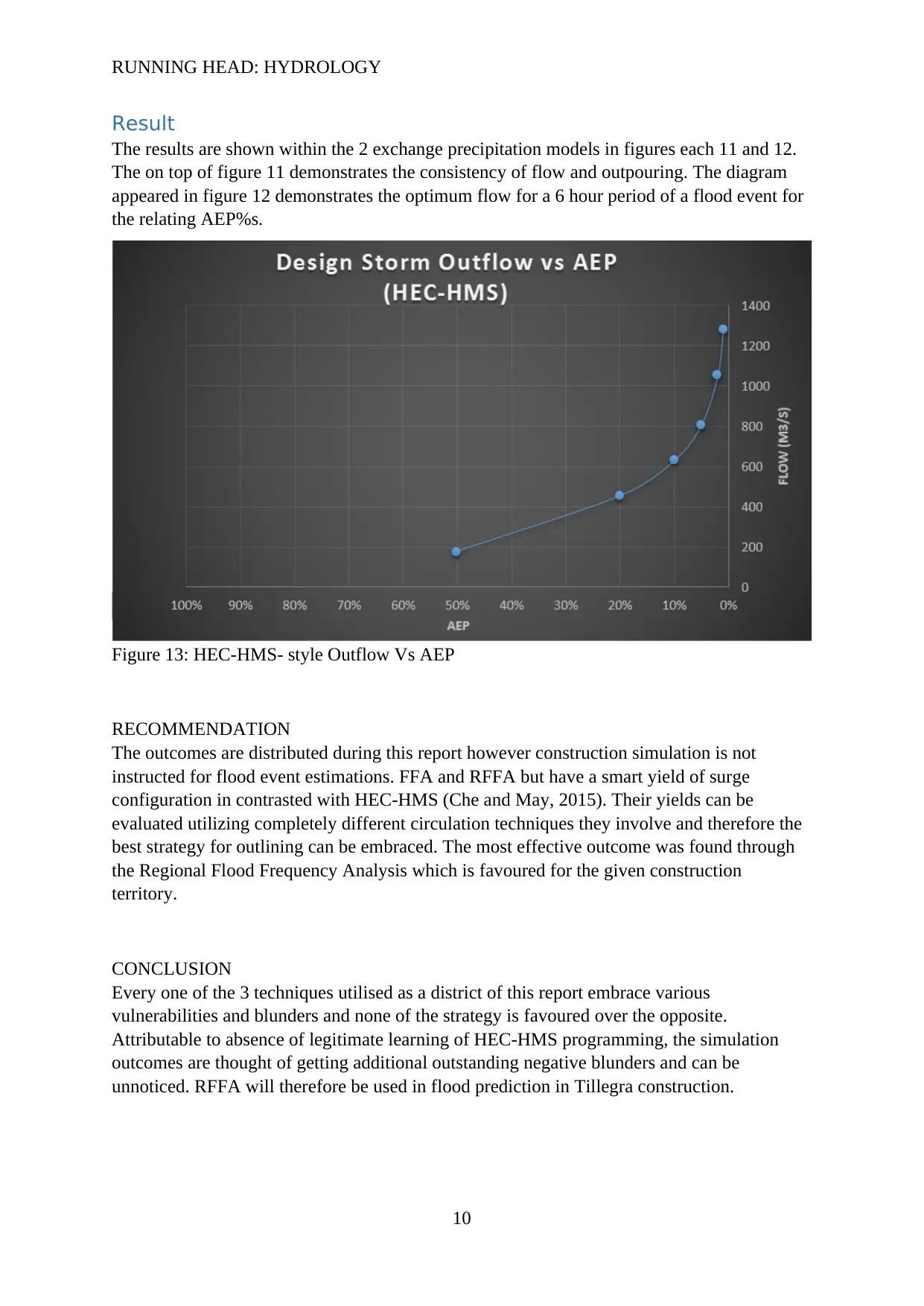
This report provides a detailed analysis of flood frequency for the design flow of a water dam (station 210011) at Tillergra on the River Williams, covering an area of 195.7 km2. The report utilizes data from 1931 to 2013 and employs three main techniques: Flood Frequency Analysis (FFA), Regional Flood Frequency Estimation (RFFA), and Catchment Simulation using HEC-HMS. The FFA method calculates design flood flows and confidence limits, while RFFA utilizes the ARR, 2013 model. Catchment simulation assesses construction response to storm events, incorporating assumptions about sub-catchments and precipitation intensity. The report includes calculations, results presented in figures and tables, and recommendations, concluding that RFFA is the most suitable method for flood prediction in the Tillegra construction due to limitations in the HEC-HMS simulation. References include sources like the Australian Bureau of Statistics and the Bureau of Meteorology.

RUNNING HEAD: HYDROLOGY
NAME
UNIT
ASSIGNMENT
ASSESSMENT NUMBER
1

RUNNING HEAD: HYDROLOGY
Table of Contents
Introduction................................................................................................................................1
Flood Frequency Analysis..........................................................................................................2
Calculations............................................................................................................................2
Result......................................................................................................................................3
Regional Flood Frequency Estimation technique......................................................................5
Calculation.............................................................................................................................5
Results....................................................................................................................................5
Catchment Simulation................................................................................................................7
Assumption............................................................................................................................7
Calculation.............................................................................................................................8
Result......................................................................................................................................9
Recommendation......................................................................................................................10
Conclusion................................................................................................................................10
References:...............................................................................................................................11
i

RUNNING HEAD: HYDROLOGY
INTRODUCTION
This report is meant to aid in the design flow of water dam (station 210011) at Tillergra on
the River Williams presently at coordinates -032.32, 151.69 that spans 195.7 km2. The
information collected for the station are for the years 1931 to 2013.
Figure 1: Williams River construction
FLOOD FREQUENCY ANALYSIS
This calculates correct information received from gauge stations and statistics are governed
by an array of assumptions.
1

RUNNING HEAD: HYDROLOGY
Figure 2: Decrease in flow maxima discovered from 1978. Global warming is presently the
presumably cause.
Calculations
The coordinates for the various positions of units plotted in the flood flow chart are found by:
P(i )= i−α
n+1−2 α
Where:
n = number of values
i = data point rank
α = 0.4 as common in Australia.
Log Pearson sort III (LPIII) chance dispersion has been utilised to play out the measurable
investigation during this report because it was the prescribed chance dissemination preceding
the draft of the modification to ARR. This chance appropriation is appropriate the knowledge
utilizing the tactic of Moments (ARR, 2013). The steps within the technique of moments are:
Xi =log10 ( Qi )
Standard dev., mean and coefficient of skewness calculation:
M = 1
n ∑
i =1
n
xi
2

RUNNING HEAD: HYDROLOGY
S= √ 1
n−1 ∑
i=1
n
( xi−M )
2
g= n
( n−1 ) ( n−2 )
∑
i=1
n
( xi−M ) 3
S3
Estimation of discharge:
log10 ( QY )=M + KY S
Where:
KY = factors of frequency
Limits of confidence:
log10 (CL5,95 ( QY ) )=log10 ( QY ) ± 1.645 δS
√ N
Here:
δ = AEP function (ARR, 2013).
Result
Figure 3 is that the curve generated when the calculation of all the mandatory applied
mathematics values of annual flows versus AEPs the FFA. Within the graph of the flow plot,
the boldness limits of ninety fifth and five-hitter are developed.
3

RUNNING HEAD: HYDROLOGY
Figure 3: Flood Frequency Curve
Having observed the graph the planning we can obtain the flood flows of interest which are
shown in Figure 4 below, at the side of confidence limits of 95% and 5%.
1 in Y(%) Qy 5% CL 95% CL
5 1399.963 819.8184 1399.963
1 2369.743 857.2829 2369.743
Figure 4: Design Flood Flows of FFA
4

RUNNING HEAD: HYDROLOGY
REGIONAL FLOOD FREQUENCY ESTIMATION TECHNIQUE
Figure 5: center of mass and Outlet of style construction with encompassing construction
location.
Figure 6: Simulated drainage area
Calculation
ARR, 2013 model package, construction information as well as the center of mass and
drainage surface were input. Also, by application of the construction form cut out and
attention-grabbing plumb lines center of mass location was calculable.
Results
The following table is generated with data given from the ARR web site. It electronically
generates the information when setting the required values relating to the layout flood waft
with appreciate to the AEPs of one hundred and twenty fifth and five-hitter. Confidence
limits of 95 and 5 are generated from the calculation.
5

RUNNING HEAD: HYDROLOGY
Figure 7: Flood frequency curve generated by ARR Website
6

RUNNING HEAD: HYDROLOGY
CATCHMENT SIMULATION
Catchment simulation is applied in the determination of future possible construction response
in the case of a storm event.
Assumption
 All the sub catchments are taken as all having equal space.
 The constant during this case is that the precipitation intensity against the interval
period.
 The time of concentration and therefore the period of time of every event are equal.
The procedure for the HEC-HMS is given by the ARR to modify the user to calculate the
precipitation depth. The HEC-HMS package is offered for downloading at
http://www.arr.org.au/ and this is often what's used with foreign information.
Concentration time is:
tc = 0.76A0.38
Where:
tc = hrs
A = sq. metres (Che and Mays, 2015).
In our case, the worth calculated is 5.66 hours and thus we'll use the 6 hours’ period in IFD.
In the time information series, the interval in use is half-hour exploitation the premise of
temporal pattern (Tahmasbine et al., 2012). The graphs are indicated below.
7

RUNNING HEAD: HYDROLOGY
Figure 10: precipitation IFD chart (Source: Bureau of Meteorology, 2013)
Calculation
When coming up with the plan hydrograph, construction simulation counts as one in every of
the technique wherever data are contribution to HEC-HMS programming. The product
naturally gauges the information and produces the ends up in figure kind, summary plotted
graph and table.
8

RUNNING HEAD: HYDROLOGY
Figure 11: Outflow-Inflow Vs Flow style
Figure 12: Peak flow design calculated using FLIKE
9

RUNNING HEAD: HYDROLOGY
Result
The results are shown within the 2 exchange precipitation models in figures each 11 and 12.
The on top of figure 11 demonstrates the consistency of flow and outpouring. The diagram
appeared in figure 12 demonstrates the optimum flow for a 6 hour period of a flood event for
the relating AEP%s.
Figure 13: HEC-HMS- style Outflow Vs AEP
RECOMMENDATION
The outcomes are distributed during this report however construction simulation is not
instructed for flood event estimations. FFA and RFFA but have a smart yield of surge
configuration in contrasted with HEC-HMS (Che and May, 2015). Their yields can be
evaluated utilizing completely different circulation techniques they involve and therefore the
best strategy for outlining can be embraced. The most effective outcome was found through
the Regional Flood Frequency Analysis which is favoured for the given construction
territory.
CONCLUSION
Every one of the 3 techniques utilised as a district of this report embrace various
vulnerabilities and blunders and none of the strategy is favoured over the opposite.
Attributable to absence of legitimate learning of HEC-HMS programming, the simulation
outcomes are thought of getting additional outstanding negative blunders and can be
unnoticed. RFFA will therefore be used in flood prediction in Tillegra construction.
10

RUNNING HEAD: HYDROLOGY
11

RUNNING HEAD: HYDROLOGY
References:
Australian Bureau of Statistics, 2016. Newcastle and Lake Macquarie, Australian
Government, viewed 9/10 /2017. http://stat.abs.gov.au/itt/r.jsp?
RegionSummary&region=111&dataset=ABS_REGIONAL_ASGS&geoconcept=REGION&
datasetASGS=ABS_REGIONAL_ASGS&datasetLGA=ABS_REGIONAL_LGA&regionLG
A=REGION&regionASGS=REGION>
Australian Rainfall & Runoff. 2013. Regional Flood Frequency Estimation Model
(Draft), Australian Government, viewed 21 May 2016. < rffe.arr.org.au>>
Bureau of Meteorology, 2015. Powells Creek catchment IFD, viewed 9/10/2017
<http://www.bom.gov.au/hydro/has/cdirswebx/cdirswebx.shtml>.
Che, D. and Mays, L.W., 2015. Development of an optimization/simulation model for real-
time flood-control operation of river-reservoirs systems. Water resources management,
29(11), pp.3987-4005.
Di Baldassarre, G. and Montanari, A., 2009. Uncertainty in river discharge observations: a
quantitative analysis. Hydrology and Earth System Sciences, 13(6), p.913.
Knebl, M.R., Yang, Z.L., Hutchison, K. and Maidment, D.R., 2005. Regional scale flood
modeling using NEXRAD rainfall, GIS, and HEC-HMS/RAS: a case study for the San
Antonio River Basin Summer 2002 storm event. Journal of Environmental Management,
75(4), pp.325-336.
Tahmasbine, H., Feyzolahpo, M., Mumipour, M. and Zakerhosei, F., 2012. Rainfall-runoff
simulation and modeling of Karun River using HEC-RAS and HEC-HMS models, Izeh
District, Iran. Journal of Applied Sciences, 12, pp.1900-1908.
12