Flood Frequency Analysis: Statistical Methods and Case Study

This project analyzes flood frequency using statistical methods applied to annual maximum flow data from Bielsdown Creek, NSW, Australia, from 1972 to 2011. It explores the concept of flood frequency, emphasizing the need for accurate frequency assessments in engineering design and flood management. The study compares statistical approaches, including the Normal, EV, LN, and LP3 distributions, and employs the Gumbel distribution for analysis. It details the methodology, including data selection, exceedance probability calculations using Gringorten's formula, and the estimation of return periods. The results section presents the analysis in an Excel worksheet format, comparing estimated and theoretical return periods and demonstrating the application of goodness-of-fit tests. The project aims to determine the most appropriate distribution model for the given data, providing insights into flood prediction and management.

INTRODUCTION
Flood frequency is an idea of the possible frequency of occurrence of a flood. It will be
insufficient in the designing of engineering works, to say that the maximum witnessed flood was,
443.06 m3/s; it will be essential to say the frequency of occurrence of this flood. Evaluating the
frequency of flood and defining the flow of flood are the key goal for hydrological exploration
and the start of flood management (Stendiger, 2012). If the 443.06 m3/s floods mentioned to
above is the size that happens on average once in every 10 years, therefore for instance any
bridge that is designed to manage with this will be under-designed by most sensible standards.
This is due to the expectation that it might not occur for long. In most cases, the design issue is
an economic one. This comes with involving capital in on-going costs of a conservatively large
structure versus the bigger risk of loss of a minor and inexpensive one.
Like in engineering works, dams and bridges, information on flood frequency is applied to
manage the use of land and settlement on flood-prone areas. Hydrological research on
determining the design flood for evaluating flood frequency is viewed using two approaches:
1. Statistical approach method- This estimates the flood quantiles by using probability
models to flood data to assess the design flood.
2. The design storm method- This uses the rainfall-runoff model and considers the rainfall
quantiles determined by frequency study as the input data (Hydrology Handbook, 1996).
Statistical approach, which uses the measured annual peak discharge data, is considered as the
standard method for approximating a flood quantile. However, a big error margin may occur in
estimating low-frequency floods if the sample size is not long enough (Klemes, 1993). Due to
the changes that occur in land use, obtaining stationarity of data for flood frequency analysis is
becoming more difficult (Beighley, 2003). This is due to changes in land use that occur with

urbanization affect the frequency of floods (Arche, 2010), studies are therefore required to be
conducted to modify the past flood data to the present condition. According to (Halcrow Group
Limited, 2008) the change in land use affects the hydrological responses of watersheds.
However, quantifying these changes is very hard. Even if flood data are available for the site of
interest, regulating the flood data measured in the past period to the present land use is difficult
and limits the calculation of correct flood quantiles.
The design storm approach is used in estimating the flood quantiles by applying rainfall quantiles
obtained from rainfall frequency analysis to the rainfall-runoff model. This method requires three
basic assumptions which include the selection of design rainfall hyetograph (rainfall duration and
time distribution), selection of antecedent soil moisture conditions before the storm occurs, and
the equality of the return periods between the rainfall quantiles and computed flood quantiles.
The assumption that the return periods are equal between rainfall quantiles and simulated flood
quantiles is not sometimes satisfactory (Adams, 1986). Many researchers have found out that the
design storm method can only produce acceptable peak discharge for a given return period if this
method is properly used (Guo, 2001).
Statistical approach in obtaining flood frequency analysis is carried out using parametric
methods in which a statistical distribution is used to fit the available data for frequency analysis
and estimation of rare events. These are normal (N), two parameter log-normal (LN2), three
parameter log-normal (LN3), two parameter gamma (G2), Pearson type III (P3), log-Pearson
type III (LP3) and Gumbel extreme value type I (G). These methods have been successfully
applied in many cases despite some disadvantages because not fitting to the experimental data
very well, or diverging from the extreme tails used earlier. Other conditions that arouse problems
with the parametric methods are involving the difficulties of approximation of the best
parameters for these approaches particularly for skewed data.
The following are ways of describing flood frequency using statistical probability.

1. Assigning the return periods to particular floods has been traditional way. It is not helpful
in trying to explain its meaning to the public. One example of a return period is when a
flood has a 1 % probability of occurring in a certain year and is thus described as a 100-
year flood event. This suggests a common but wrong notion that there should be an
interval of 100 years between events. The probability of having two 100-year floods
within 10 years is nearly 10 %.
2. Another one is the annual exceedance probability (AEP). This is the probability that a
specific flood size will occur in one given year. As with example above, the 100-year
flood will have an AEP of 1 %. Describing the probability using this approach is better
as compared to the first one.
3. The probable maximum flood (PMF) concept that is mostly applied in engineering. This
is also similar to the two methods used above, and it often uses the 100-year per 1 %
probability, since most designs are based on this. It is unlikely that PMF implies a lower
probability than 1 %, and values as low as 0.1 % used in its applications. Trying to
derive a PMF is very risky unless there is a very long record.
Q can used to define the flood variable of interest, the annual maximum flow, in which the flow
Q exceeds a threshold q*. The inference of the pth quantile, Qpt (quantile) of Q, for year t,
conditional on some set of m climatic indices (or other predictors), Xt = [xt x2t _ _ _ xmt], is of
interest. To do this, an estimate of the conditional probability density function f(Qt|Xt), or the
conditional distribution function F(Qt|Xt) from the historical data {Qt, Xt, t = 1. . .n}:
F p (Qt ∨Xt )=∫
−∞
Q pt
f ( Qt |Xt ) dQ= p Equation 1a
Qpt =F p
−1 (Qt ∨X t ) Equation 1b
The conventional way to estimate the conditional distribution function F (Qt|Xt) assums that the
joint probability density function f(Qt, Xt) follows a certain distribution to estimate its

parameters. Quantile approximations obtained from this method differ widely since it depends on
the nature of the tails of the conditional probability density function (Qt|Xt). (Jain, 2000) tried to
overcome this by assuming f(Qt|Xt) to be lognormal, with its mean and variance changing in
time conditional on the state of ENSO and PDO over a 30 year moving window.
Quantile regression is a parametric approach that is used to estimate conditional quantiles. It
works by minimizing the total of asymmetrically weighted absolute deviation by giving different
weights for positive and negative residuals using simple optimization techniques. The benefit of
using this approach is that it is easy and can be extended even under nonlinear situations
(Koenkar, 1996). This study considers the parametric quantile regression method in comparing
non-parametric approach in estimating flood quantiles. The performance of the above methods is
compared on a synthetic data set that can be evaluated for a potential application in delivering
seasonal flood predictions in a hydrologic basin.

METHODOLOGY
The annual maximum flow data from 1972 to 2011 for Station 204017 is selected analysis. This
station is at Bielsdown Creek at Dorrigo Number 2 & Number 3 in NSW State.
This study is considering the application of four probability distributions, i.e. Normal, EV, LN
and LP3 in flood modelling, and illustrates the applicability of Goodness of Fit test procedures in
determining which distributional model is best for the given data. Table 1 below gives the
Probability Density Function (PDF) with the conforming flood estimator (QT) of N, EV1, LN
and LP3 distributions used in modelling flood data. Goodness of Fit tests is based either on
Cumulative Distribution Function (CDF) or on PDF. Χ2- test is based on PDF, and A2 and KS
tests are based on CDF approach; and hence belong to the class of distance tests. Adding on the
above, Dindex is used to measure the adequacy of fitting distributions to the recorded AMD data
in the upper tail region. The test gives weightage of the upper most six data points only, rather
than the data points at lower levels. This is in accordance of the selected objective of testing the
appropriate distribution for approximation of flood.
Data was computed in a excel spreadsheet and ranked from largest to smallest and introduced a
column for rank in and values inputted in decreasing order using the excel pull down menu to do
this. A q column in the excel sheet was created, Gringorten's plotting position formula is used in
order to estimate the exceedance probabilities associated with historic observation as shown
below:
q= i−a
N +1−2 a Equation 2
Where,
q = Exceedance probability associated with a specific observation;

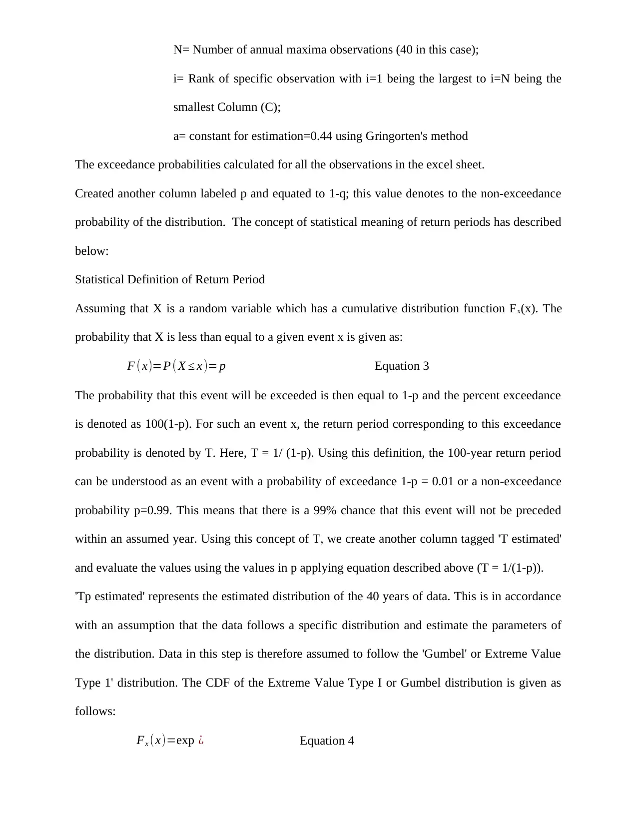
N= Number of annual maxima observations (40 in this case);
i= Rank of specific observation with i=1 being the largest to i=N being the
smallest Column (C);
a= constant for estimation=0.44 using Gringorten's method
The exceedance probabilities calculated for all the observations in the excel sheet.
Created another column labeled p and equated to 1-q; this value denotes to the non-exceedance
probability of the distribution. The concept of statistical meaning of return periods has described
below:
Statistical Definition of Return Period
Assuming that X is a random variable which has a cumulative distribution function Fx(x). The
probability that X is less than equal to a given event x is given as:
F ( x)=P ( X ≤ x )= p Equation 3
The probability that this event will be exceeded is then equal to 1-p and the percent exceedance
is denoted as 100(1-p). For such an event x, the return period corresponding to this exceedance
probability is denoted by T. Here, T = 1/ (1-p). Using this definition, the 100-year return period
can be understood as an event with a probability of exceedance 1-p = 0.01 or a non-exceedance
probability p=0.99. This means that there is a 99% chance that this event will not be preceded
within an assumed year. Using this concept of T, we create another column tagged 'T estimated'
and evaluate the values using the values in p applying equation described above (T = 1/(1-p)).
'Tp estimated' represents the estimated distribution of the 40 years of data. This is in accordance
with an assumption that the data follows a specific distribution and estimate the parameters of
the distribution. Data in this step is therefore assumed to follow the 'Gumbel' or Extreme Value
Type 1' distribution. The CDF of the Extreme Value Type I or Gumbel distribution is given as
follows:
Fx (x)=exp ¿ Equation 4

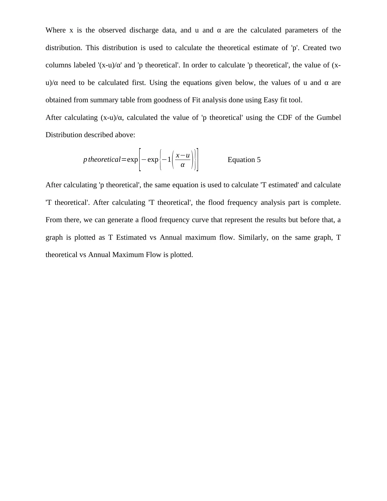
Where x is the observed discharge data, and u and α are the calculated parameters of the
distribution. This distribution is used to calculate the theoretical estimate of 'p'. Created two
columns labeled '(x-u)/α' and 'p theoretical'. In order to calculate 'p theoretical', the value of (x-
u)/α need to be calculated first. Using the equations given below, the values of u and α are
obtained from summary table from goodness of Fit analysis done using Easy fit tool.
After calculating (x-u)/α, calculated the value of 'p theoretical' using the CDF of the Gumbel
Distribution described above:
p theoretical=exp [−exp {−1 ( x−u
α ) }] Equation 5
After calculating 'p theoretical', the same equation is used to calculate 'T estimated' and calculate
'T theoretical'. After calculating 'T theoretical', the flood frequency analysis part is complete.
From there, we can generate a flood frequency curve that represent the results but before that, a
graph is plotted as T Estimated vs Annual maximum flow. Similarly, on the same graph, T
theoretical vs Annual Maximum Flow is plotted.

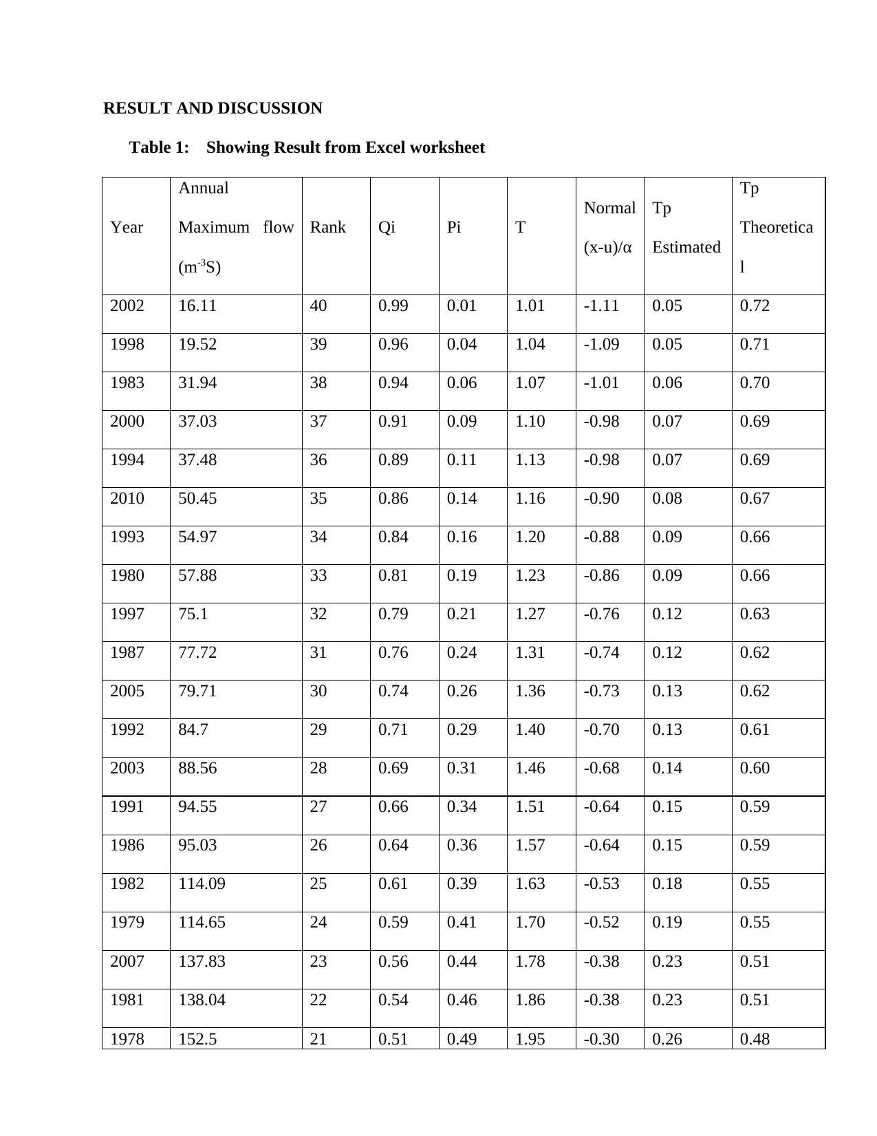
RESULT AND DISCUSSION
Table 1: Showing Result from Excel worksheet
Year
Annual
Maximum flow
(m-3S)
Rank Qi Pi T
Normal
(x-u)/α
Tp
Estimated
Tp
Theoretica
l
2002 16.11 40 0.99 0.01 1.01 -1.11 0.05 0.72
1998 19.52 39 0.96 0.04 1.04 -1.09 0.05 0.71
1983 31.94 38 0.94 0.06 1.07 -1.01 0.06 0.70
2000 37.03 37 0.91 0.09 1.10 -0.98 0.07 0.69
1994 37.48 36 0.89 0.11 1.13 -0.98 0.07 0.69
2010 50.45 35 0.86 0.14 1.16 -0.90 0.08 0.67
1993 54.97 34 0.84 0.16 1.20 -0.88 0.09 0.66
1980 57.88 33 0.81 0.19 1.23 -0.86 0.09 0.66
1997 75.1 32 0.79 0.21 1.27 -0.76 0.12 0.63
1987 77.72 31 0.76 0.24 1.31 -0.74 0.12 0.62
2005 79.71 30 0.74 0.26 1.36 -0.73 0.13 0.62
1992 84.7 29 0.71 0.29 1.40 -0.70 0.13 0.61
2003 88.56 28 0.69 0.31 1.46 -0.68 0.14 0.60
1991 94.55 27 0.66 0.34 1.51 -0.64 0.15 0.59
1986 95.03 26 0.64 0.36 1.57 -0.64 0.15 0.59
1982 114.09 25 0.61 0.39 1.63 -0.53 0.18 0.55
1979 114.65 24 0.59 0.41 1.70 -0.52 0.19 0.55
2007 137.83 23 0.56 0.44 1.78 -0.38 0.23 0.51
1981 138.04 22 0.54 0.46 1.86 -0.38 0.23 0.51
1978 152.5 21 0.51 0.49 1.95 -0.30 0.26 0.48

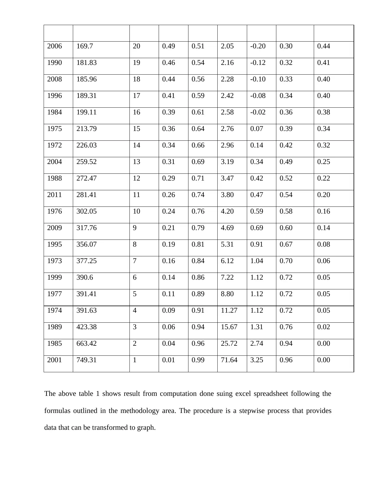
2006 169.7 20 0.49 0.51 2.05 -0.20 0.30 0.44
1990 181.83 19 0.46 0.54 2.16 -0.12 0.32 0.41
2008 185.96 18 0.44 0.56 2.28 -0.10 0.33 0.40
1996 189.31 17 0.41 0.59 2.42 -0.08 0.34 0.40
1984 199.11 16 0.39 0.61 2.58 -0.02 0.36 0.38
1975 213.79 15 0.36 0.64 2.76 0.07 0.39 0.34
1972 226.03 14 0.34 0.66 2.96 0.14 0.42 0.32
2004 259.52 13 0.31 0.69 3.19 0.34 0.49 0.25
1988 272.47 12 0.29 0.71 3.47 0.42 0.52 0.22
2011 281.41 11 0.26 0.74 3.80 0.47 0.54 0.20
1976 302.05 10 0.24 0.76 4.20 0.59 0.58 0.16
2009 317.76 9 0.21 0.79 4.69 0.69 0.60 0.14
1995 356.07 8 0.19 0.81 5.31 0.91 0.67 0.08
1973 377.25 7 0.16 0.84 6.12 1.04 0.70 0.06
1999 390.6 6 0.14 0.86 7.22 1.12 0.72 0.05
1977 391.41 5 0.11 0.89 8.80 1.12 0.72 0.05
1974 391.63 4 0.09 0.91 11.27 1.12 0.72 0.05
1989 423.38 3 0.06 0.94 15.67 1.31 0.76 0.02
1985 663.42 2 0.04 0.96 25.72 2.74 0.94 0.00
2001 749.31 1 0.01 0.99 71.64 3.25 0.96 0.00
The above table 1 shows result from computation done suing excel spreadsheet following the
formulas outlined in the methodology area. The procedure is a stepwise process that provides
data that can be transformed to graph.

1 10
0
2
4
6
8
10
12
Annual Maximum flow (m-
3S
Tp Estimated
Tp Theoretical
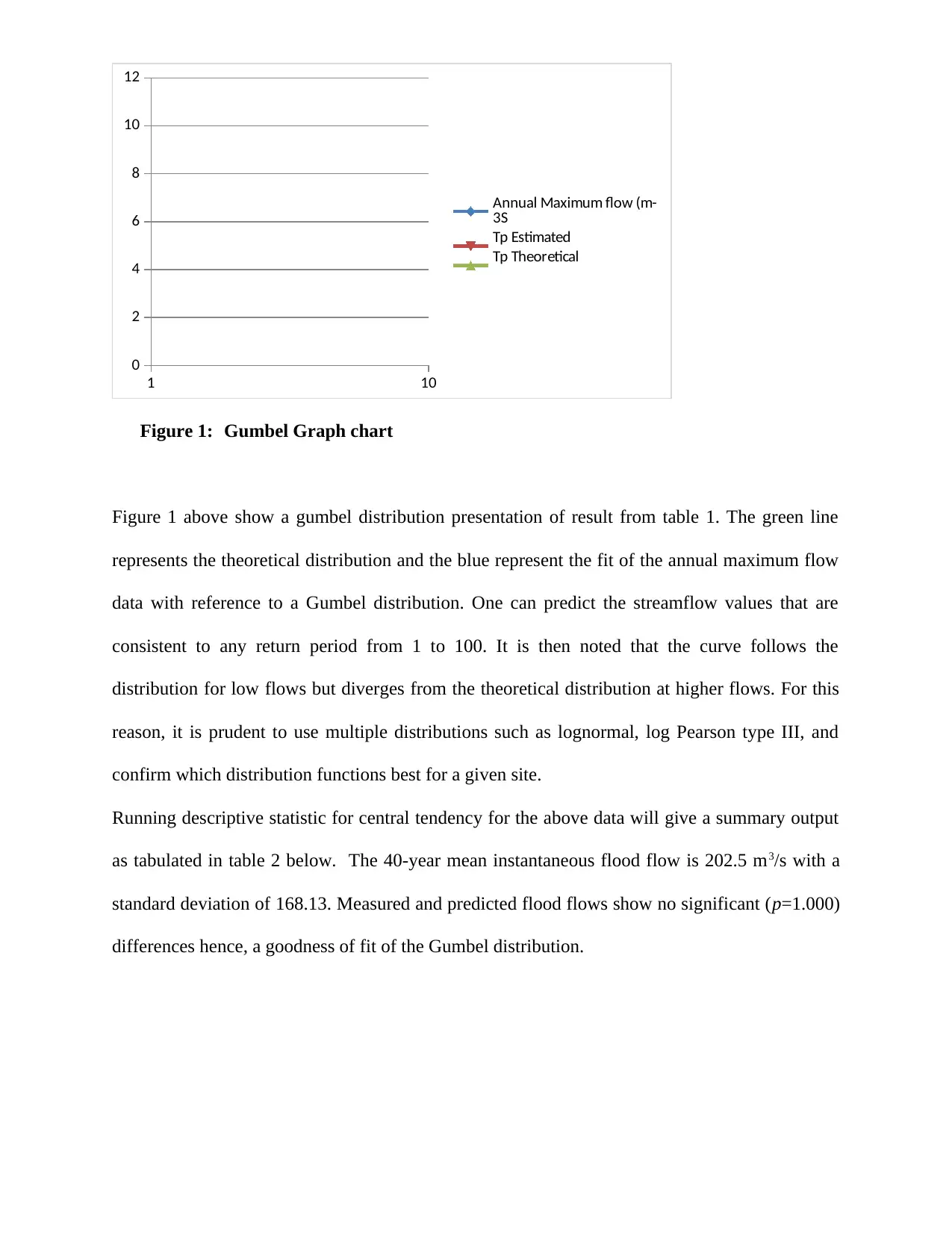
Figure 1: Gumbel Graph chart
Figure 1 above show a gumbel distribution presentation of result from table 1. The green line
represents the theoretical distribution and the blue represent the fit of the annual maximum flow
data with reference to a Gumbel distribution. One can predict the streamflow values that are
consistent to any return period from 1 to 100. It is then noted that the curve follows the
distribution for low flows but diverges from the theoretical distribution at higher flows. For this
reason, it is prudent to use multiple distributions such as lognormal, log Pearson type III, and
confirm which distribution functions best for a given site.
Running descriptive statistic for central tendency for the above data will give a summary output
as tabulated in table 2 below. The 40-year mean instantaneous flood flow is 202.5 m3/s with a
standard deviation of 168.13. Measured and predicted flood flows show no significant (p=1.000)
differences hence, a goodness of fit of the Gumbel distribution.

Table 2: Table for Measure of central tendency
Measure of Central
Tendency
Annual
Maximum flow
(m-3S
Tp Estimated Tp Theoretical
Mean 202.50 0.3496 0.4075
Standard Error 26.58 0.0422 0.0386
Median 161.10 0.2784 0.4575
Standard Deviation 168.13 0.2671 0.2439
Sample Variance 28267.82 0.0714 0.0595
Kurtosis 2.38 -0.6092 -1.3124
Skewness 1.45 0.7359 -0.4140
Range 733.20 0.9137 0.7189
Minimum 16.11 0.0483 0.0000
Maximum 749.31 0.9621 0.7189
Confidence
Level(95.0%)
53.77 0.0854 0.0780
Table 3: Goodness of Fit - Summary
Distribution
Kolmogorov
Smirnov
Anderson
Darling
Chi-Squared
Statistic Rank Statistic Rank Statistic Rank
1 Gen. Extreme Valu 0.09066 4 0.31684 3 2.1941 4

e
2 Log-Pearson 3 0.06017 1 0.18186 1 0.51948 1
3 Lognormal 0.08447 3 0.32748 4 1.036 2
4 Lognormal (3P) 0.07301 2 0.2663 2 1.1327 3
5 Normal 0.1338 5 1.4295 5 3.5106 5
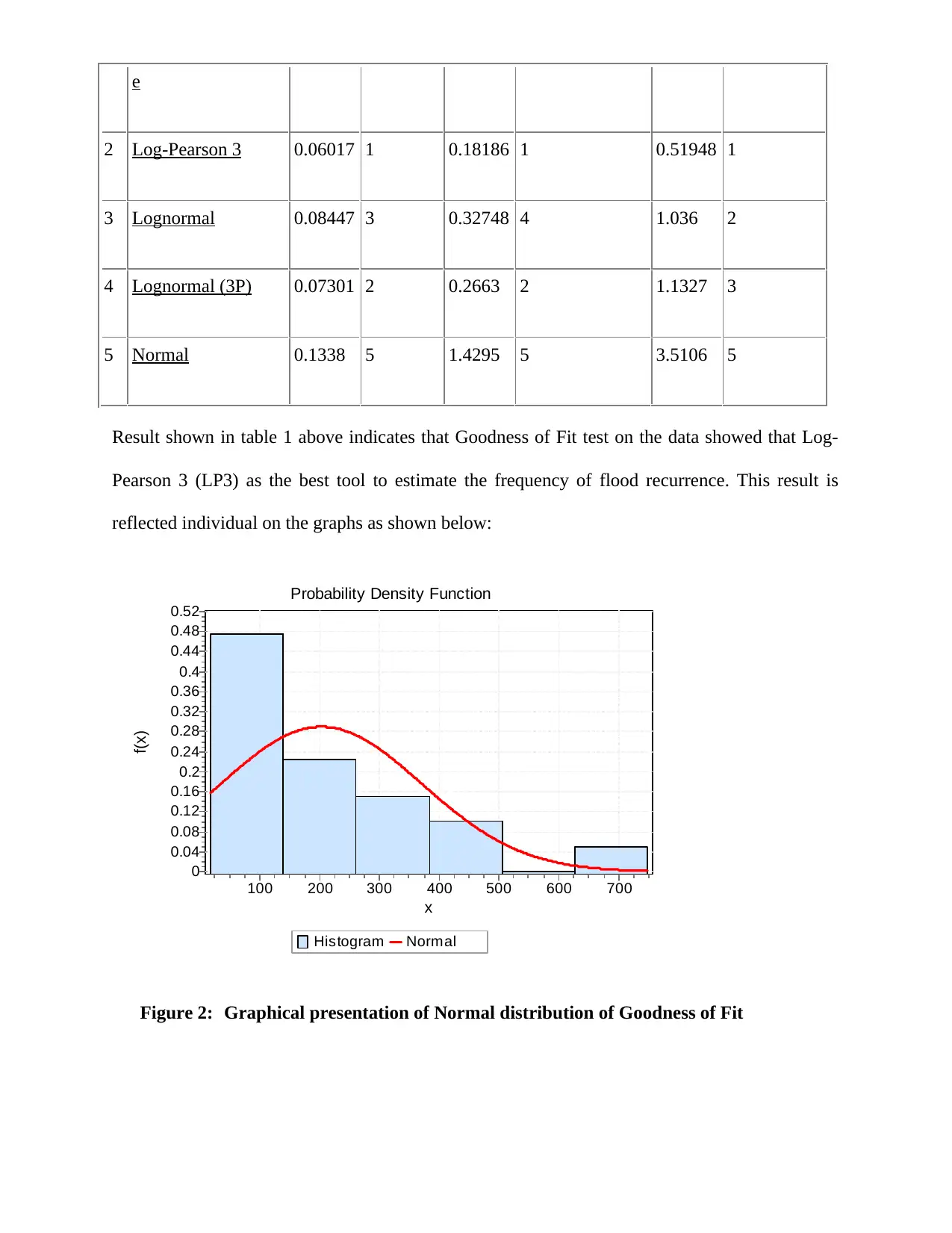
Result shown in table 1 above indicates that Goodness of Fit test on the data showed that Log-
Pearson 3 (LP3) as the best tool to estimate the frequency of flood recurrence. This result is
reflected individual on the graphs as shown below:
Probability Density Function
Histogram Normal
x
700600500400300200100
f(x)
0.52
0.48
0.44
0.4
0.36
0.32
0.28
0.24
0.2
0.16
0.12
0.08
0.04
0
Figure 2: Graphical presentation of Normal distribution of Goodness of Fit