Advanced Thermal & Fluid Engineering: CFD Simulation of Cylinder

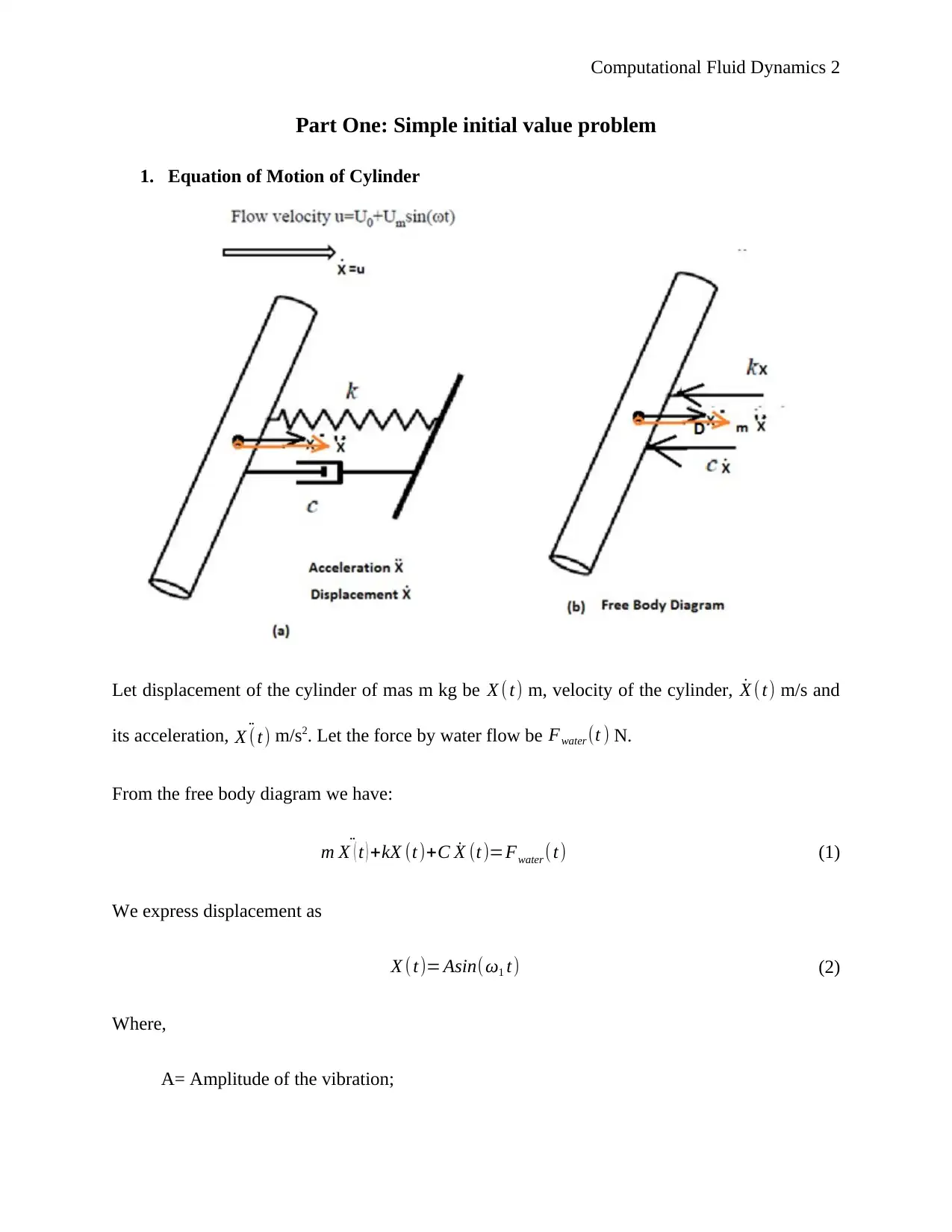
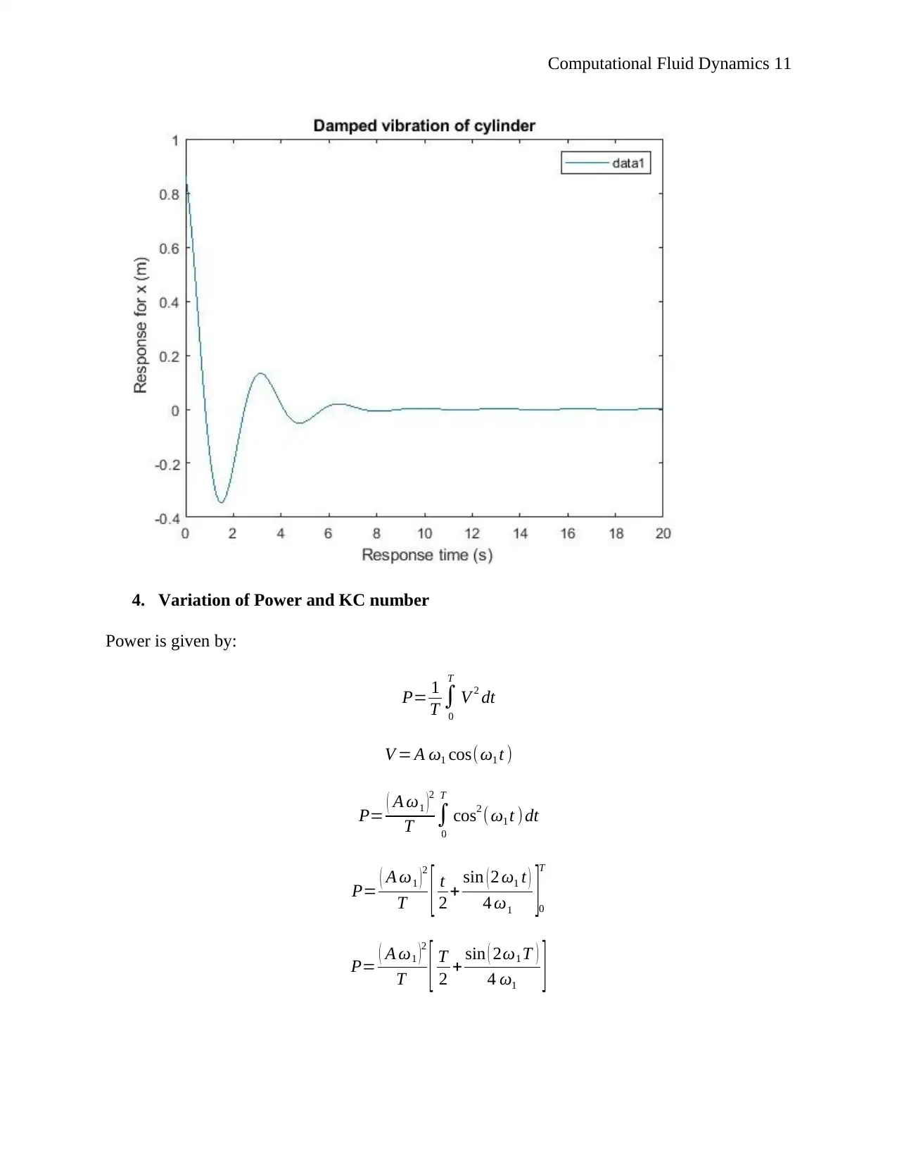
This project provides a detailed solution to a Computational Fluid Dynamics (CFD) assignment involving two primary parts: a simple initial value problem concerning the equation of motion of a cylinder and a one-dimensional convection-diffusion problem. The first part includes deriving the equation of motion for a cylinder subjected to water flow, developing a numerical method using Euler-Runge Kutta and Finite Difference Method (FDM) to predict the cylinder's vibration, presenting Matlab code for simulation, and analyzing the variation of power with the Keulegan-Carpenter (KC) number and damping coefficient (C). It also includes time history plots for displacement, velocity, and power. The second part addresses the convection-diffusion equation, solved using finite difference methods. Desklib offers students access to this solved assignment and many other resources for academic support.

Computational Fluid Dynamics 1
COMPUTATIONAL FLUID DYNAMICS
By Name
Course
Professor
University
City/State
Date

Computational Fluid Dynamics 2
Part One: Simple initial value problem
1. Equation of Motion of Cylinder
Let displacement of the cylinder of mas m kg be X (t) m, velocity of the cylinder, ˙X ( t) m/s and
its acceleration, ¨X (t) m/s2. Let the force by water flow be Fwater (t ) N.
From the free body diagram we have:
m ¨X ( t ) +kX (t)+C ˙X (t)=Fwater (t) (1)
We express displacement as
X (t)= Asin(ω1 t) (2)
Where,
A= Amplitude of the vibration;

Computational Fluid Dynamics 3
ω1= Angular velocity of the vibration, rad/s.
We therefore have velocity as:
˙X (t)= A ω1 cos (ω1 t ) (3)
And Acceleration as:
¨X (t)=− A ω1
2 sin (ω1 t) (4)
¨X (t)=−ω1
2 X (t) (5)
Force, Fwater, on the cylinder is expressed as:
Fwater ( t ) =CA md
d V r
dt + ρC D Ap
2 |V r|V r (6)
Where,
CD=Coefficient of drag;
C A=Coefficient of inertia;
Ap= Surface area of the cylinder experiencing drag, m2;
|V r|= Magnitude of vibration velocity;
V r=Velocity of flow relative to cylinder, m/s; same as u- ˙X (t );
md=Displacement fluid mass, kg;
ρ= Density of water, kgm-3;
u= Flow velocity, m/s.

Computational Fluid Dynamics 4
Using Equation 6 we have:-
Fwater ( t ) =CA md
d V r
dt + ρC D Ap
2 |V r|V r (7)
u=U0 +Um sin ( ωt )
V r =u− ˙X (t)
V r =U0 +Um sin ( ωt )− A ω1 cos (ω1 t )
d V r
dt =Um ωcos ( ωt )+ A ω1
2 sin(ω1 t)
Fwater ( t ) =CA md U m ωcos ( ωt ) +C A md A ω1
2 sin(ω1 t)+ ρC D A p
2 |V r|( U0 +Um sin ( ωt ) − A ω1 cos(ω1 t ) )
(8)
Equation of motion becomes:
m ¨X ( t ) +kX (t)+C ˙X (t )=C A md Um ωcos ( ωt ) ¿+ CA md A ω1
2 sin(ω1 t)+ ρCD A p
2 |V r|(U 0+ Um sin ( ωt )− A ω1 cos
Which becomes:
( m+C A md ) ¨X ( t ) + ( C+ ρC D Ap
2 |V r|) ˙X +kX ( t ) =C A md Um ωcos ( ωt ) ¿+ ρC D A p
2 |V r|( U0 +Um sin ( ωt ) )
(9)
We will use Euler – Runge Kutta method.
Runge Kutta method is of the form
dy
dx =f ( x , y ) , y ( 0 ) , y0 (10)

Computational Fluid Dynamics 5
Since Runge Kutta is applicable in first order ODE, we shall use it with Euler’s method.
Euler’s method is derived from Taylor’s expansion as in steps below.
X ( x0 +h ) =X ( x0 ) +h X x ( x0 ) +O ( h2 ) (11)
We have
X x ( x0 ) = X ( x0 +h )− X ( x0 )
h +O ( h2 )
h
Taking h=∆ x we have
X x ( x0 ) = X ( x0 +h )− X ( x0 )
∆ x +O ∆ t
Neglecting Oh we have
X x ( x0 ) ≈ X ( x0+ ∆ t ) −X ( x0 )
∆ t (12)
For higher orders, the Euler’s method is given by
X ( t , x0 +∆ t ) =X ( t , x0 ) +∆ t Xx ( t , x0 ) + ( ∆ t ) 2
2 ! Xxx ( t , x0 ) +… (13)
The first two terms of the series gives Taylor’s series and form Runge-Kutta first order method.
Truncating gives Equation 13 gives Runge-Kutta second order formula:
X ( t , x0 +∆ t ) =X ( t , x0 ) +∆ t Xx (t , x0 ) + ( ∆ t )2
2 ! Xxx ( t , x0 )
This was summarized by Runge Kutta as:

Computational Fluid Dynamics 6
yi+1 = yi+ ( a1 k1 +a2 k2 ) h
Where,
k1 =f ( xi , yi)
k 2=f ( xi + p1 h , yi + q11 k 1 h)
Finite Difference approximation
X x ( x0 ) = Xi+1− Xi−1
∆ t (13)
X xx ( t , x0 )= Xi+ 1−2 Xi+ Xi−1
( ∆ t )2 (14)
From the oscillatory component of the equation;
Ft ( t0 ) = Fi+ 1−Fi−1
2 ∆ t (15)
The FDM approximation of equation of motion becomes
( m+C A md ) ¨X ( t )+ (C+ ρC D Ap
2 |V r|) ˙X +kX ( t )=g(t , x ) (16)
Where k = Xx
X
FDM approximation
( m+C A md ) ( Xi +1−2 Xi + Xi−1
( ∆ t )2 ) +( C+ ρC D A p
2 |V r|)( Xi+1− Xi−1
∆ t ) +k Xi−1=Gi−1 (17)

Computational Fluid Dynamics 7
2. Numerical Method for Predicting Vibration of Cylinder
From Equation 9:
We have:
( m+C A md ) ( Xi +1−2 Xi + Xi−1
( ∆ t )2 ) +k X i−1 =0 (18)
We have
( Xi +1−2 Xi+ Xi−1
( ∆ t )2 )≈ ω1
2 Xi−1 (19)
− ( m+C A md ) ω1
2 Xi−1 +k Xi−1=0 (20)
( m+C A md ) ω1
2 =k (21)
From Equation 21 we have
ω1
2= k
m+C A md
(22)
Natural frequency of cylinder vibration is given by:

Computational Fluid Dynamics 8
ω1= √ k
m+C A md
(23)
And that for damping coefficient we have:
2 ζ ω1 ˙X ( t ) =2 ζ ω1 ( Xi +1−Xi−1
∆ t )= ( C+ ρC D Ap
2 |V r|)( Xi +1−Xi−1
∆ t )
Giving
2 ζ=
C+ ρC D Ap
2 |V r|
ω1
ζ = 2C+ ρC D A p|V r|
4 ω1
¿ 2C +ρC D A p |V r|
4 √ k
m+ CA md
(24)
Damped natural frequency is given by:
ωd= √ 1−ζ2 ω1
3. Matlab Coding
Using the given values, we have:
clear all;
close all;
clc;
% Defining variables

Computational Fluid Dynamics 9
k=200; % spring stiffness in N/m
m=50; % mass of cylinder in kg
CA=1; % Inertia coefficient
D=0.12; % diameter of cylinder in m
w=2; % Angular velocity of oscillatory flow
L=1; % length of cylinder m
rho=1.024; % density of water
tf=100; % Duration of vibration in seconds
x0=0.01; % initial displacement of cylinder
v0=0.01; %initial velocity of cylinder
Um=1.2; % Amplitude of oscillatory flow
U0=0.1*Um; % Steady-state velocity of water, m/s
C=1.0; % Damping coefficient in Ns/m
Cd=1.8; % Coefficient of drag
%% Calculating projected area
Ap=D*L;
%% Calculating the displaced mass
md=(pi/4)*D^2*L*rho;
% Natural frequency of undamped vibration
wn=sqrt(k/(m+CA*md));
% Period
T=2*pi/wn;

Computational Fluid Dynamics 10
%% Initializing time increment
t=0:tf/1000:tf;
for t=1:tf
V=sin(wn*t);
u=U0-Um*sin(w*t);
Vr=u-V; % velocity of flow relative to cylinder
Vmag=sqrt(u^2+V^2);
%% Damping ratio zeta
zeta=(2*C+rho*Cd*Ap*Vmag)/(4*wn);
%% Damped natural frequency
wd=sqrt(1-zeta*zeta)*wn;
%% Calculating resultant amplitude, a, phase difference phi, and displacement, x
a=1/(sqrt((C+(rho*Cd*Ap*Vmag/2))^2+(k-(m+CA*md)*wn^2)^2));
phi=atan(C+(rho*Cd*Ap*Vmag/2)/(k-(m+CA*md)*wn^2));
t=0:0.1:20;
x=a*exp(-zeta*wn*t).*sin(wd*t+phi);
plot(t,x)
title('Damped vibration of cylinder')
ylabel(' Response for x (m)')
xlabel(' Response time (s)')
end

Computational Fluid Dynamics 11
4. Variation of Power and KC number
Power is given by:
P= 1
T ∫
0
T
V 2 dt
V = A ω1 cos(ω1 t )
P= ( A ω1 )2
T ∫
0
T
cos2 (ω1 t ) dt
P= ( A ω1 ) 2
T [ t
2 + sin ( 2 ω1 t )
4 ω1 ]0
T
P= ( A ω1 )
2
T [ T
2 + sin ( 2ω1 T )
4 ω1 ]

Computational Fluid Dynamics 12
P= ( A ω1 )2
[ 1
2 + sin ( 2 ω1 T )
4 ω1 T ]
P= ( A ω1 )2
[ 1
2 + sin ( 2 ω1 T )
8 π ]
KC =U m
D T
T = KC∗D
Um
Matlab Code
clear all;
close all;
clc;
% Defining variables
A=1; % Amplitude of displacement
KC=2:2:20;
C=100; % Coefficient of damping, Ns/m
k=KC/C;
Um=1.2; % amplitude of oscillatory velocity
m=50; % mass of cylinder
CA=1; % Coefficient of inertia