Analysis of Forced Convection Heat Transfer Experiment - G100 Module
VerifiedAdded on 2022/08/09
|12
|2492
|452
Practical Assignment
AI Summary
This report details a forced convection heat transfer experiment conducted using the TD1 Forced Convection Heat Transfer apparatus. The objective was to determine the convective heat transfer coefficient, velocity distribution, and temperature distribution of air flowing through a heated pipe. The experiment involved measuring parameters like atmospheric pressure, temperature, orifice pressure drop, fan pressure rise, and heater voltage and current. Data was collected to calculate the air mass flow rate, air density, and heat transfer coefficient. Velocity and temperature profiles across the pipe diameter were also obtained using a pitot tube and thermocouples. The results, including calculated values for heat transfer coefficient and velocity, are presented in tables and graphs. The discussion section analyzes the temperature and velocity distributions, comparing them to theoretical profiles and discussing potential sources of error. The experiment successfully demonstrated the principles of forced convection and provided a practical application of heat transfer theory.
Forced Convection Heat Transfer
Objective:
1) To determine the convective heat transfer coefficient for forced convection.
2) To determine the velocity and temperature distribution in fluid flow.
Introduction:
In many engineering applications, applications of forced convection heat transfer is found.
Thus it is important to have knowledge of this topic specially while designing heat-
exchangers.
Heat Exchanger is a device used to exchange of heat between two fluids at different
temperatures. The fluid at higher temperature loses heat and the fluid at colder temperature
gains heat and its temperature rises. Thus the heat transfer takes from hot fluid to the cold
fluid.
The transfer of heat can occur in 3 different modes, Conduction, Convection and Radiation.
The key principles acting in heat exchangers are convection and conductive heat transfer. In
this case, heat transfer by radiation is negligible in comparison to other two modes of heat
transfer. In this experiment conduction occurs as the heat from the electric heating tape
passes through the copper pipe wall and then heat transferred to the moving fluid is made
through forced convection.
Theory
In a fluid when there is bulk fluid motion, then the heat transfer takes place by convection.
When there is no bulk motion, then heat transfer occurs by conduction.
Convection involves fluid motion as well as heat conduction.
Heat transfer takes place from the heated surface to fluid passing over the surface have lower
temperature. This is illustrated in figure 1. The fluid motion when caused by a fan or pump,
results in forced convection heat transfer. By Newton’s Law of cooling, this forced
convection heat transfer is given by (Bahrami, n.d.):
˙qconv =h As ( T s−T ∞ ) (W/m2) (1)
Where h = convective heat transfer coefficient (W/m2K)
T ∞= fluid average temperature ( oC)
Ts = pipe surface temperature ( oC)
Paraphrase This Document
Need a fresh take? Get an instant paraphrase of this document with our AI Paraphraser
Calculation of mass flow rate
To determine the mass flow rate an orifice plate in the pipe connects to a manometer on the
instrumentation panel. The equation related to the orifice plate is given as
˙m=0.00365∗√ ( horiface(mm))/(ρair ) (2)
Where
horifice is the manometer reading (mm), and
ρair is the local air density (kg/m3)
To determine the air density at the orifice we use the equation of state
𝑝=𝜌×𝑅×𝑇 (3)
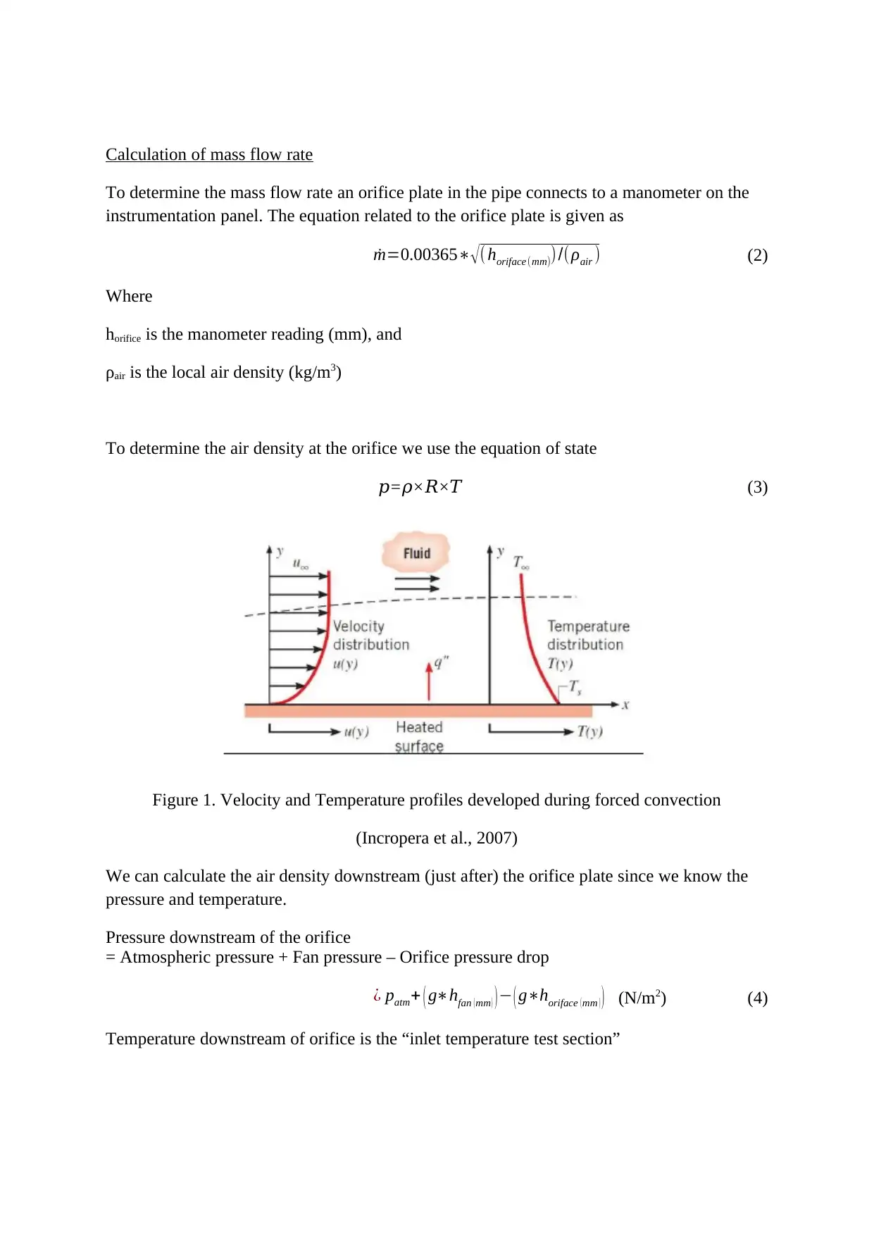
Figure 1. Velocity and Temperature profiles developed during forced convection
(Incropera et al., 2007)
We can calculate the air density downstream (just after) the orifice plate since we know the
pressure and temperature.
Pressure downstream of the orifice
= Atmospheric pressure + Fan pressure – Orifice pressure drop
¿ patm+ ( g∗hfan ( mm ) ) − ( g∗horiface ( mm ) ) (N/m2) (4)
Temperature downstream of orifice is the “inlet temperature test section”
To determine the mass flow rate an orifice plate in the pipe connects to a manometer on the
instrumentation panel. The equation related to the orifice plate is given as
˙m=0.00365∗√ ( horiface(mm))/(ρair ) (2)
Where
horifice is the manometer reading (mm), and
ρair is the local air density (kg/m3)
To determine the air density at the orifice we use the equation of state
𝑝=𝜌×𝑅×𝑇 (3)
Figure 1. Velocity and Temperature profiles developed during forced convection
(Incropera et al., 2007)
We can calculate the air density downstream (just after) the orifice plate since we know the
pressure and temperature.
Pressure downstream of the orifice
= Atmospheric pressure + Fan pressure – Orifice pressure drop
¿ patm+ ( g∗hfan ( mm ) ) − ( g∗horiface ( mm ) ) (N/m2) (4)
Temperature downstream of orifice is the “inlet temperature test section”
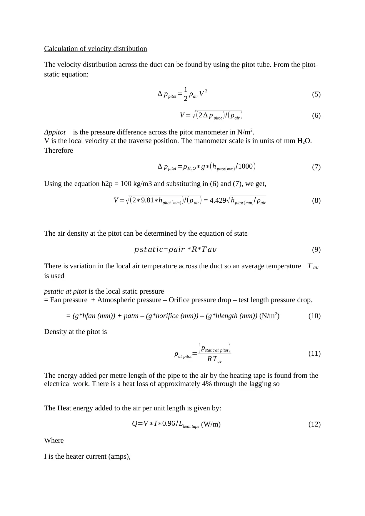
Calculation of velocity distribution
The velocity distribution across the duct can be found by using the pitot tube. From the pitot-
static equation:
∆ ppitot = 1
2 ρair V 2 (5)
V = √(2 ∆ p pitot )/( ρair ) (6)
Δppitot is the pressure difference across the pitot manometer in N/m2.
V is the local velocity at the traverse position. The manometer scale is in units of mm H2O.
Therefore
∆ ppitot =ρH 2O∗g∗(h pitot(mm) /1000) (7)
Using the equation h2p = 100 kg/m3 and substituting in (6) and (7), we get,
V = √ (2∗9.81∗hpitot (mm))/(ρair) = 4.429 √ hpitot (mm)/ ρair (8)
The air density at the pitot can be determined by the equation of state
𝑝𝑠𝑡𝑎𝑡𝑖𝑐=𝜌𝑎𝑖𝑟 *𝑅*𝑇𝑎𝑣 (9)
There is variation in the local air temperature across the duct so an average temperature 𝑇𝑎𝑣
is used
pstatic at pitot is the local static pressure
= Fan pressure + Atmospheric pressure – Orifice pressure drop – test length pressure drop.
= (g*hfan (mm)) + patm – (g*horifice (mm)) – (g*hlength (mm)) (N/m2) (10)
Density at the pitot is
ρat pitot= ( pstatic at pitot )
R Tav
(11)
The energy added per metre length of the pipe to the air by the heating tape is found from the
electrical work. There is a heat loss of approximately 4% through the lagging so
The Heat energy added to the air per unit length is given by:
Q=V ∗I∗0.96 /Lheat tape (W/m) (12)
Where
I is the heater current (amps),
⊘ This is a preview!⊘
Do you want full access?
Subscribe today to unlock all pages.
Trusted by 1+ million students worldwide
V is the heater voltage (volts)
and
Lheattape is the length of the pipe wrapped with heating tape (m)
Since L is 1.75m then
˙Q=0.55V ∗I (W/m) (13)
Using the Newton’s law of cooling , we determine the Heat transferred by convection from
the wall
˙Q=h Aw ( T w−T AV ) (14)
Where:
Aw is the inner surface area of the pipe from start of heating to pitot tube
h is the convective heat transfer coefficient (W/m2.K)
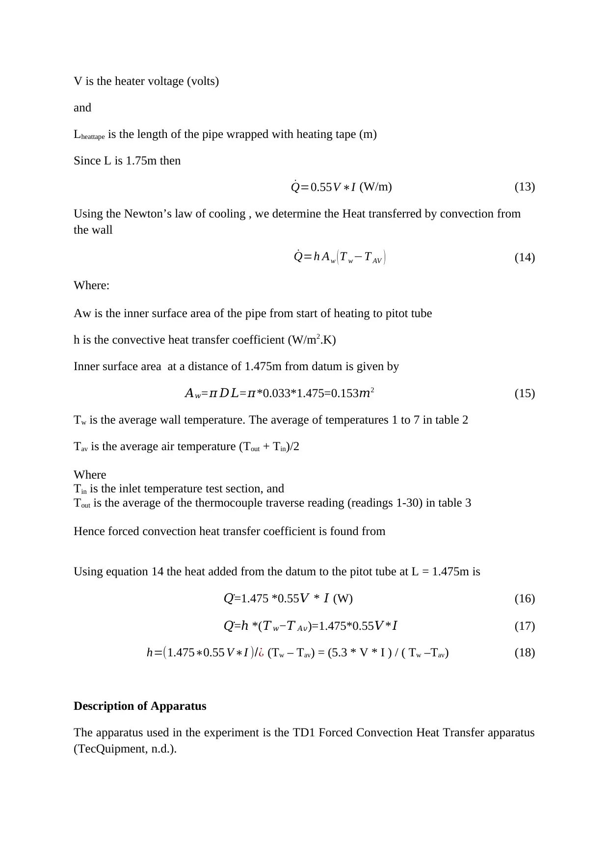
Inner surface area at a distance of 1.475m from datum is given by
𝐴𝑤=𝜋𝐷𝐿=𝜋*0.033*1.475=0.153𝑚2 (15)
Tw is the average wall temperature. The average of temperatures 1 to 7 in table 2
Tav is the average air temperature (Tout + Tin)/2
Where
Tin is the inlet temperature test section, and
Tout is the average of the thermocouple traverse reading (readings 1-30) in table 3
Hence forced convection heat transfer coefficient is found from
Using equation 14 the heat added from the datum to the pitot tube at L = 1.475m is
𝑄̇=1.475 *0.55𝑉 * 𝐼 (W) (16)
𝑄̇= *(ℎ 𝑇𝑤−𝑇𝐴𝑣)=1.475*0.55𝑉*𝐼 (17)
h=(1.475∗0.55 V∗I )/¿ (Tw – Tav) = (5.3 * V * I ) / ( Tw –Tav) (18)
Description of Apparatus
The apparatus used in the experiment is the TD1 Forced Convection Heat Transfer apparatus
(TecQuipment, n.d.).
and
Lheattape is the length of the pipe wrapped with heating tape (m)
Since L is 1.75m then
˙Q=0.55V ∗I (W/m) (13)
Using the Newton’s law of cooling , we determine the Heat transferred by convection from
the wall
˙Q=h Aw ( T w−T AV ) (14)
Where:
Aw is the inner surface area of the pipe from start of heating to pitot tube
h is the convective heat transfer coefficient (W/m2.K)
Inner surface area at a distance of 1.475m from datum is given by
𝐴𝑤=𝜋𝐷𝐿=𝜋*0.033*1.475=0.153𝑚2 (15)
Tw is the average wall temperature. The average of temperatures 1 to 7 in table 2
Tav is the average air temperature (Tout + Tin)/2
Where
Tin is the inlet temperature test section, and
Tout is the average of the thermocouple traverse reading (readings 1-30) in table 3
Hence forced convection heat transfer coefficient is found from
Using equation 14 the heat added from the datum to the pitot tube at L = 1.475m is
𝑄̇=1.475 *0.55𝑉 * 𝐼 (W) (16)
𝑄̇= *(ℎ 𝑇𝑤−𝑇𝐴𝑣)=1.475*0.55𝑉*𝐼 (17)
h=(1.475∗0.55 V∗I )/¿ (Tw – Tav) = (5.3 * V * I ) / ( Tw –Tav) (18)
Description of Apparatus
The apparatus used in the experiment is the TD1 Forced Convection Heat Transfer apparatus
(TecQuipment, n.d.).
Paraphrase This Document
Need a fresh take? Get an instant paraphrase of this document with our AI Paraphraser
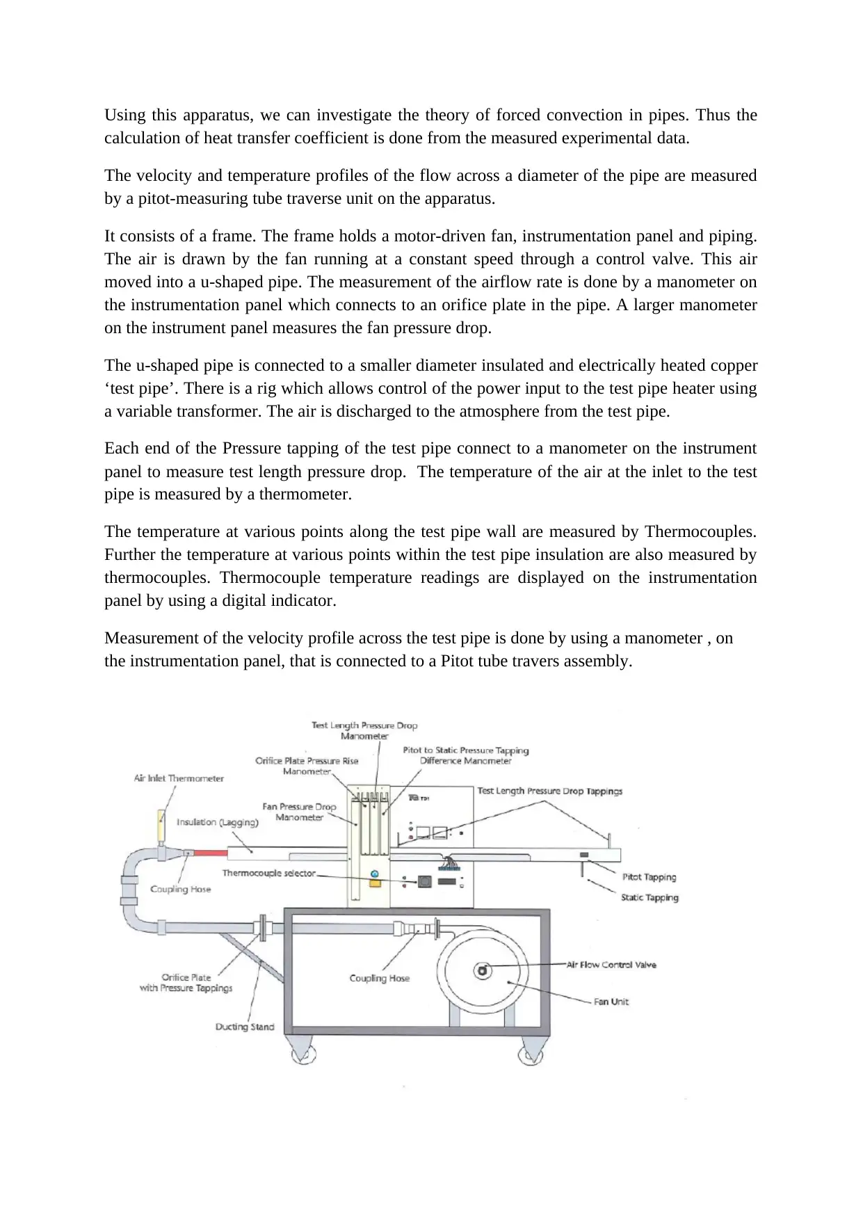
Using this apparatus, we can investigate the theory of forced convection in pipes. Thus the
calculation of heat transfer coefficient is done from the measured experimental data.
The velocity and temperature profiles of the flow across a diameter of the pipe are measured
by a pitot-measuring tube traverse unit on the apparatus.
It consists of a frame. The frame holds a motor-driven fan, instrumentation panel and piping.
The air is drawn by the fan running at a constant speed through a control valve. This air
moved into a u-shaped pipe. The measurement of the airflow rate is done by a manometer on
the instrumentation panel which connects to an orifice plate in the pipe. A larger manometer
on the instrument panel measures the fan pressure drop.
The u-shaped pipe is connected to a smaller diameter insulated and electrically heated copper
‘test pipe’. There is a rig which allows control of the power input to the test pipe heater using
a variable transformer. The air is discharged to the atmosphere from the test pipe.
Each end of the Pressure tapping of the test pipe connect to a manometer on the instrument
panel to measure test length pressure drop. The temperature of the air at the inlet to the test
pipe is measured by a thermometer.
The temperature at various points along the test pipe wall are measured by Thermocouples.
Further the temperature at various points within the test pipe insulation are also measured by
thermocouples. Thermocouple temperature readings are displayed on the instrumentation
panel by using a digital indicator.
Measurement of the velocity profile across the test pipe is done by using a manometer , on
the instrumentation panel, that is connected to a Pitot tube travers assembly.
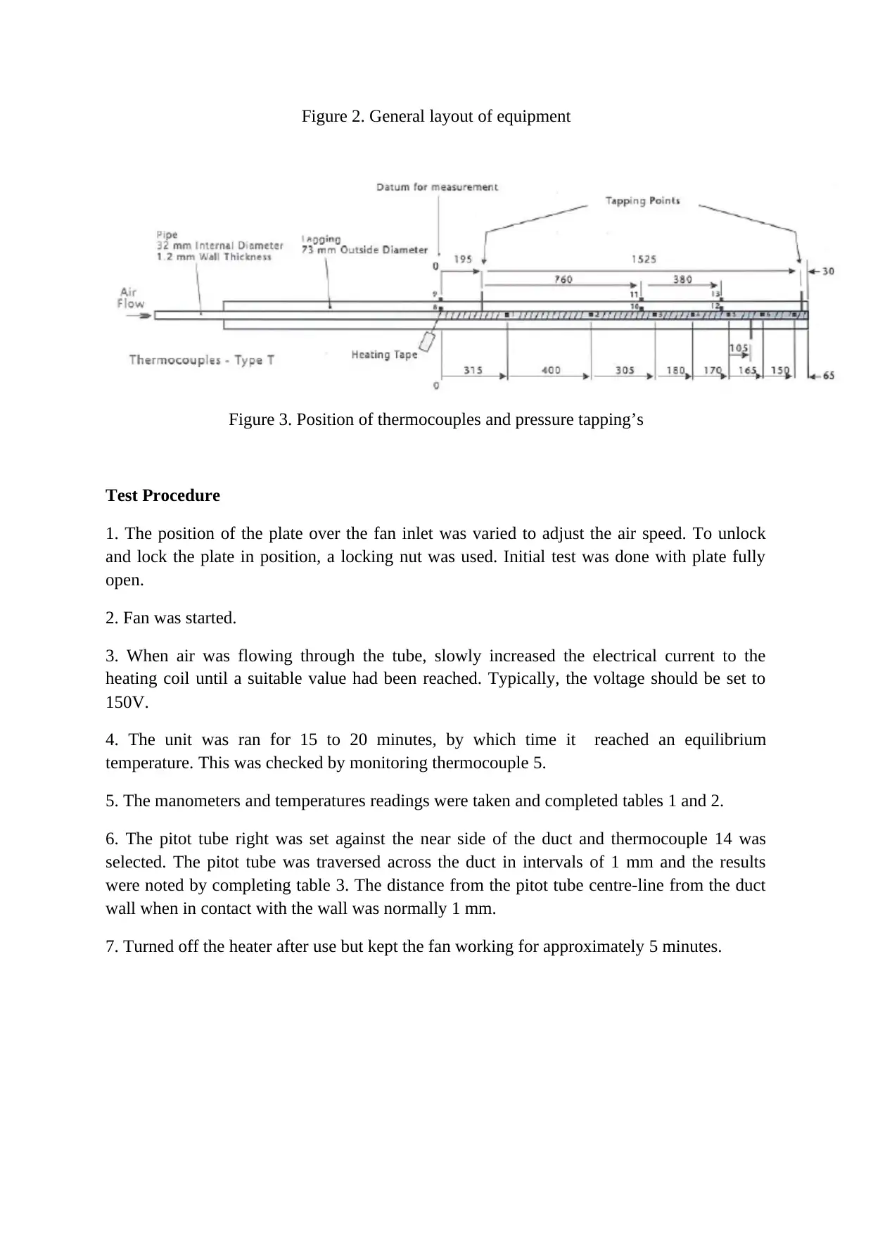
Figure 2. General layout of equipment
Figure 3. Position of thermocouples and pressure tapping’s
Test Procedure
1. The position of the plate over the fan inlet was varied to adjust the air speed. To unlock
and lock the plate in position, a locking nut was used. Initial test was done with plate fully
open.
2. Fan was started.
3. When air was flowing through the tube, slowly increased the electrical current to the
heating coil until a suitable value had been reached. Typically, the voltage should be set to
150V.
4. The unit was ran for 15 to 20 minutes, by which time it reached an equilibrium
temperature. This was checked by monitoring thermocouple 5.
5. The manometers and temperatures readings were taken and completed tables 1 and 2.
6. The pitot tube right was set against the near side of the duct and thermocouple 14 was
selected. The pitot tube was traversed across the duct in intervals of 1 mm and the results
were noted by completing table 3. The distance from the pitot tube centre-line from the duct
wall when in contact with the wall was normally 1 mm.
7. Turned off the heater after use but kept the fan working for approximately 5 minutes.
⊘ This is a preview!⊘
Do you want full access?
Subscribe today to unlock all pages.
Trusted by 1+ million students worldwide
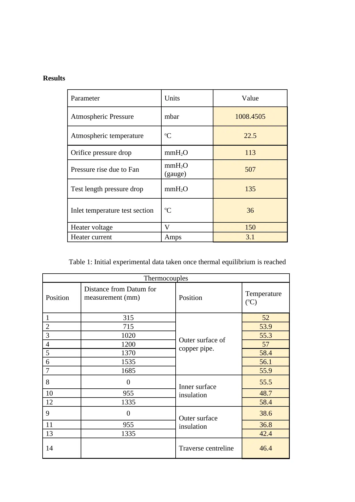
Results
Parameter Units Value
Atmospheric Pressure mbar 1008.4505
Atmospheric temperature oC 22.5
Orifice pressure drop mmH2O 113
Pressure rise due to Fan mmH2O
(gauge) 507
Test length pressure drop mmH2O 135
Inlet temperature test section oC 36
Heater voltage V 150
Heater current Amps 3.1
Table 1: Initial experimental data taken once thermal equilibrium is reached
Thermocouples
Position
Distance from Datum for
measurement (mm) Position Temperature
(oC)
1 315
Outer surface of
copper pipe.
52
2 715 53.9
3 1020 55.3
4 1200 57
5 1370 58.4
6 1535 56.1
7 1685 55.9
8 0 Inner surface
insulation
55.5
10 955 48.7
12 1335 58.4
9 0 Outer surface
insulation
38.6
11 955 36.8
13 1335 42.4
14 Traverse centreline 46.4
Paraphrase This Document
Need a fresh take? Get an instant paraphrase of this document with our AI Paraphraser
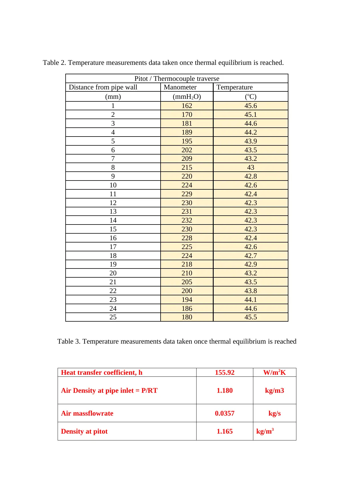
Table 2. Temperature measurements data taken once thermal equilibrium is reached.
Pitot / Thermocouple traverse
Distance from pipe wall Manometer Temperature
(mm) (mmH2O) (oC)
1 162 45.6
2 170 45.1
3 181 44.6
4 189 44.2
5 195 43.9
6 202 43.5
7 209 43.2
8 215 43
9 220 42.8
10 224 42.6
11 229 42.4
12 230 42.3
13 231 42.3
14 232 42.3
15 230 42.3
16 228 42.4
17 225 42.6
18 224 42.7
19 218 42.9
20 210 43.2
21 205 43.5
22 200 43.8
23 194 44.1
24 186 44.6
25 180 45.5
Table 3. Temperature measurements data taken once thermal equilibrium is reached
Heat transfer coefficient, h 155.92 W/m2K
Air Density at pipe inlet = P/RT 1.180 kg/m3
Air massflowrate 0.0357 kg/s
Density at pitot 1.165 kg/m3
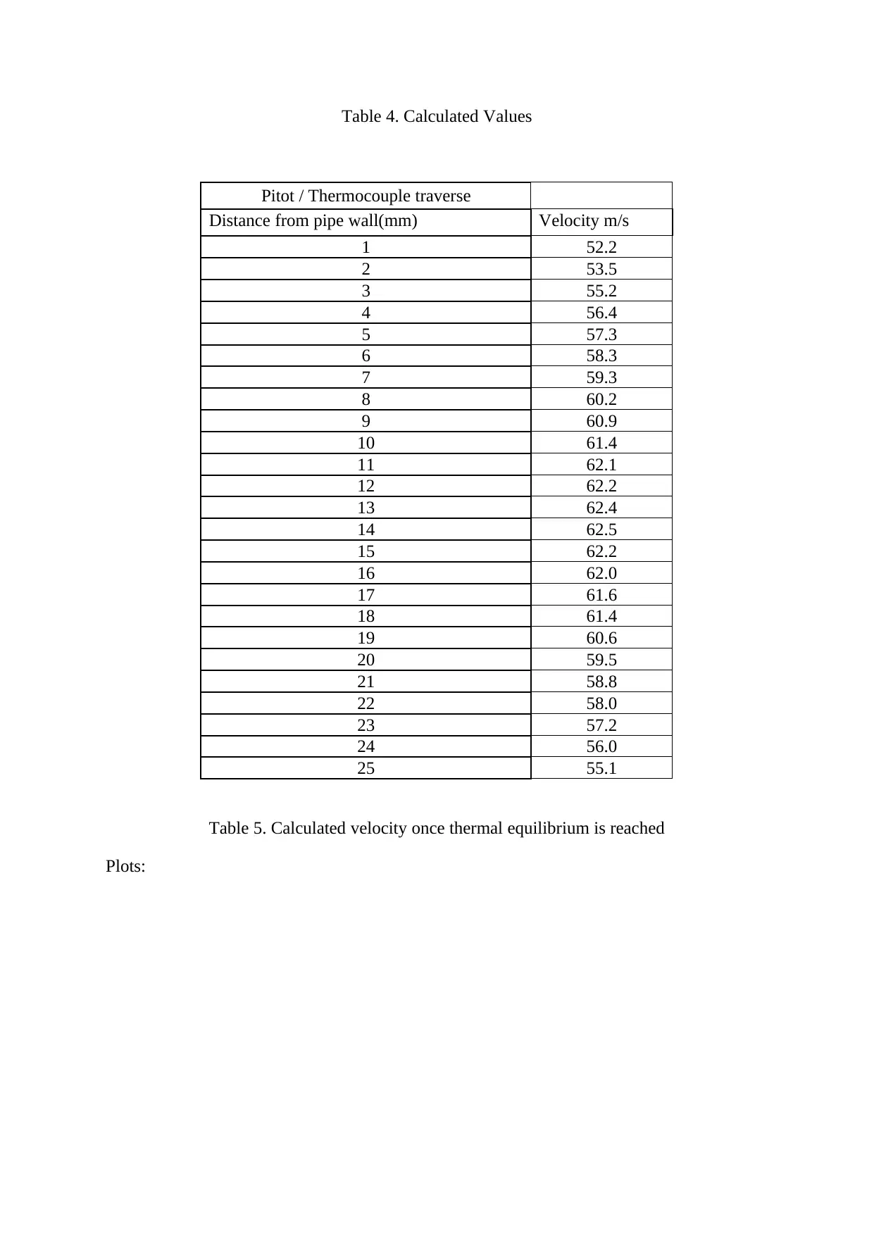
Table 4. Calculated Values
Pitot / Thermocouple traverse
Distance from pipe wall(mm) Velocity m/s
1 52.2
2 53.5
3 55.2
4 56.4
5 57.3
6 58.3
7 59.3
8 60.2
9 60.9
10 61.4
11 62.1
12 62.2
13 62.4
14 62.5
15 62.2
16 62.0
17 61.6
18 61.4
19 60.6
20 59.5
21 58.8
22 58.0
23 57.2
24 56.0
25 55.1
Table 5. Calculated velocity once thermal equilibrium is reached
Plots:
⊘ This is a preview!⊘
Do you want full access?
Subscribe today to unlock all pages.
Trusted by 1+ million students worldwide
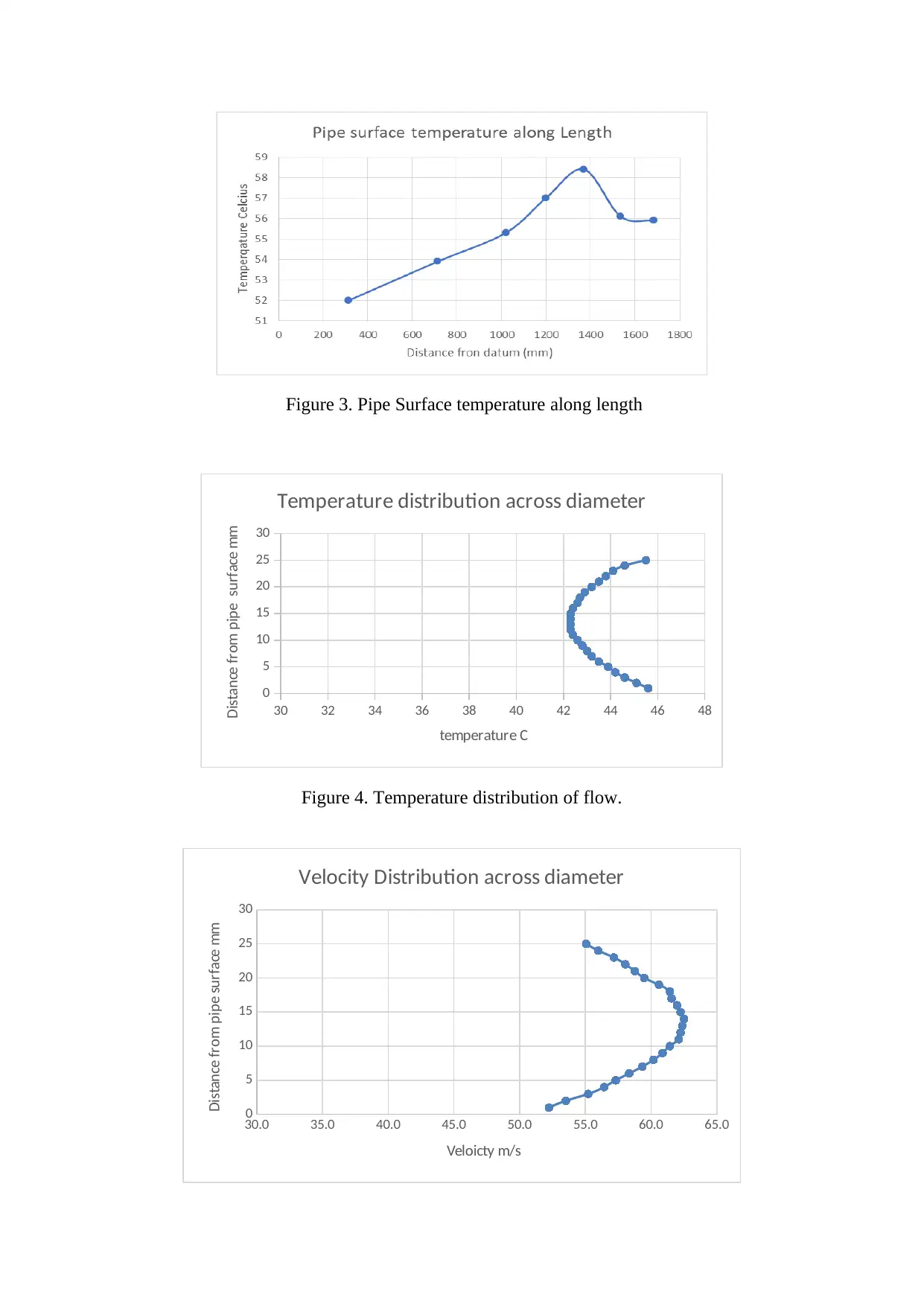
Figure 3. Pipe Surface temperature along length
30 32 34 36 38 40 42 44 46 48
0
5
10
15
20
25
30
Temperature distribution across diameter
temperature C
Distance from pipe surface mm
Figure 4. Temperature distribution of flow.
30.0 35.0 40.0 45.0 50.0 55.0 60.0 65.0
0
5
10
15
20
25
30
Velocity Distribution across diameter
Veloicty m/s
Distance from pipe surface mm
Paraphrase This Document
Need a fresh take? Get an instant paraphrase of this document with our AI Paraphraser
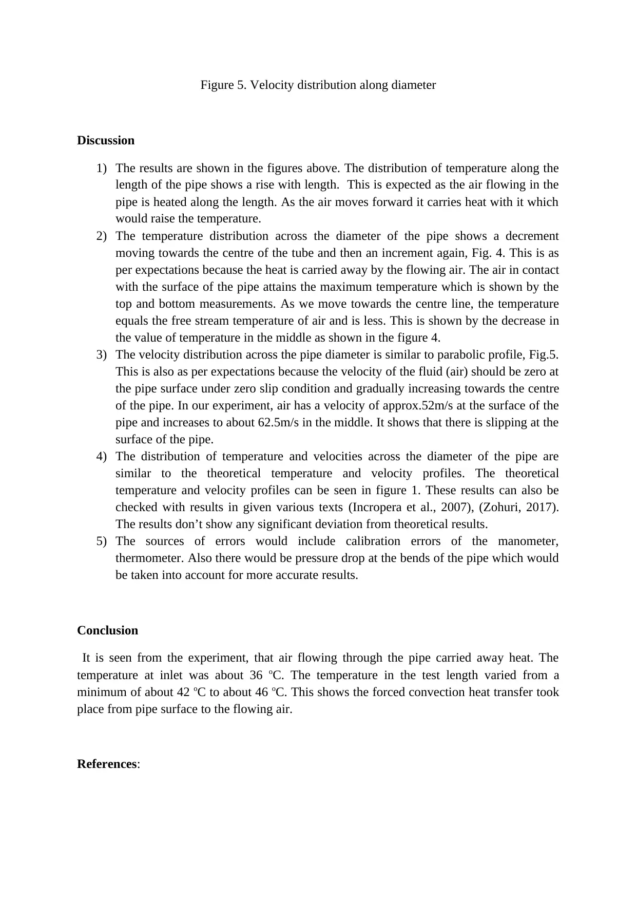
Figure 5. Velocity distribution along diameter
Discussion
1) The results are shown in the figures above. The distribution of temperature along the
length of the pipe shows a rise with length. This is expected as the air flowing in the
pipe is heated along the length. As the air moves forward it carries heat with it which
would raise the temperature.
2) The temperature distribution across the diameter of the pipe shows a decrement
moving towards the centre of the tube and then an increment again, Fig. 4. This is as
per expectations because the heat is carried away by the flowing air. The air in contact
with the surface of the pipe attains the maximum temperature which is shown by the
top and bottom measurements. As we move towards the centre line, the temperature
equals the free stream temperature of air and is less. This is shown by the decrease in
the value of temperature in the middle as shown in the figure 4.
3) The velocity distribution across the pipe diameter is similar to parabolic profile, Fig.5.
This is also as per expectations because the velocity of the fluid (air) should be zero at
the pipe surface under zero slip condition and gradually increasing towards the centre
of the pipe. In our experiment, air has a velocity of approx.52m/s at the surface of the
pipe and increases to about 62.5m/s in the middle. It shows that there is slipping at the
surface of the pipe.
4) The distribution of temperature and velocities across the diameter of the pipe are
similar to the theoretical temperature and velocity profiles. The theoretical
temperature and velocity profiles can be seen in figure 1. These results can also be
checked with results in given various texts (Incropera et al., 2007), (Zohuri, 2017).
The results don’t show any significant deviation from theoretical results.
5) The sources of errors would include calibration errors of the manometer,
thermometer. Also there would be pressure drop at the bends of the pipe which would
be taken into account for more accurate results.
Conclusion
It is seen from the experiment, that air flowing through the pipe carried away heat. The
temperature at inlet was about 36 oC. The temperature in the test length varied from a
minimum of about 42 oC to about 46 oC. This shows the forced convection heat transfer took
place from pipe surface to the flowing air.
References:
Bahrami, M. (n.d.). Forced Convection Heat Transfer. [ebook] Available at:
https://www.sfu.ca/~mbahrami/ENSC%20388/Notes/Forced%20Convection.pdf [Accessed 1
Mar. 2020].
INCROPERA, F., DEWITT, D., BERGMAN, T. and LAVINE, A. (2007). Fundamentals of
Heat and Mass Transfer. 6th ed. USA: John Wiley and Sons.
TecQuipment. (n.d.). FORCED CONVECTION HEAT TRANSFER. [online] Available at:
https://www.tecquipment.com/forced-convection-heat-transfer [Accessed 1 Mar. 2020].
Zohuri, B. (2017). Forced Convection Heat Transfer. [online] www.researchgate.com.
Available at:
https://www.researchgate.net/publication/318039452_Forced_Convection_Heat_Transfer
[Accessed 1 Mar. 2020].
⊘ This is a preview!⊘
Do you want full access?
Subscribe today to unlock all pages.
Trusted by 1+ million students worldwide
1 out of 12
Related Documents


Your All-in-One AI-Powered Toolkit for Academic Success.
+13062052269
info@desklib.com
Available 24*7 on WhatsApp / Email
![[object Object]](/_next/static/media/star-bottom.7253800d.svg)
Unlock your academic potential
Copyright © 2020–2026 A2Z Services. All Rights Reserved. Developed and managed by ZUCOL.