Case Study: Forecasting Techniques, Error Analysis, and Model Fitting

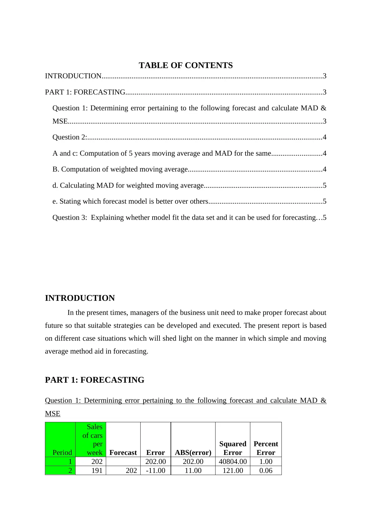
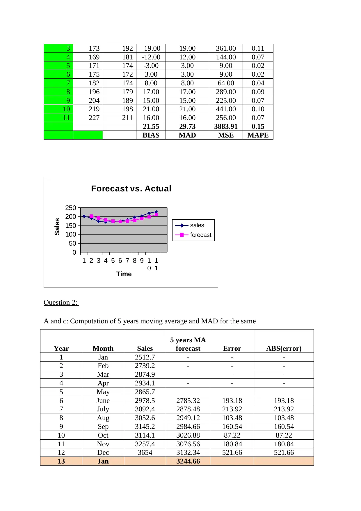
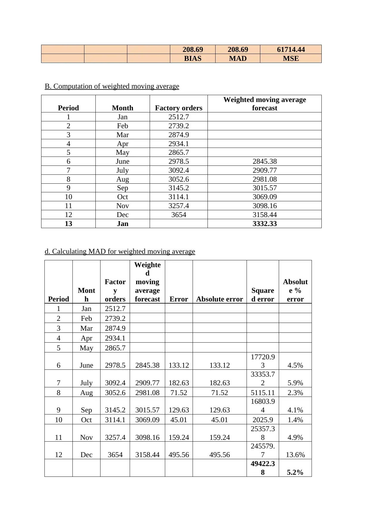
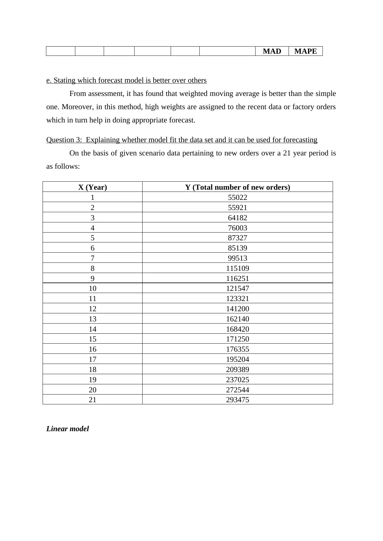
This case study delves into various forecasting techniques, encompassing error analysis and model comparison. It begins by calculating error metrics such as MAD, MSE, and percent error for a given forecast. The analysis extends to the application of moving average methods, including both simple and weighted moving averages, and evaluating their performance. The study further explores model fitting, examining how well different models align with a dataset and their suitability for forecasting future trends. This involves the interpretation of linear and polynomial models, with a focus on the goodness of fit and the use of statistical measures like regression to predict values. Ultimately, the case study provides a comprehensive overview of forecasting methods, error analysis, and model evaluation, highlighting the strengths and weaknesses of each approach.

Forecasting / Case study

TABLE OF CONTENTS
INTRODUCTION......................................................................................................................3
PART 1: FORECASTING.........................................................................................................3
Question 1: Determining error pertaining to the following forecast and calculate MAD &
MSE........................................................................................................................................3
Question 2:.............................................................................................................................4
A and c: Computation of 5 years moving average and MAD for the same...........................4
B. Computation of weighted moving average........................................................................4
d. Calculating MAD for weighted moving average...............................................................5
e. Stating which forecast model is better over others.............................................................5
Question 3: Explaining whether model fit the data set and it can be used for forecasting...5
INTRODUCTION
In the present times, managers of the business unit need to make proper forecast about
future so that suitable strategies can be developed and executed. The present report is based
on different case situations which will shed light on the manner in which simple and moving
average method aid in forecasting.
PART 1: FORECASTING
Question 1: Determining error pertaining to the following forecast and calculate MAD &
MSE
Period
Sales
of cars
per
week Forecast Error ABS(error)
Squared
Error
Percent
Error
1 202 202.00 202.00 40804.00 1.00
2 191 202 -11.00 11.00 121.00 0.06

3 173 192 -19.00 19.00 361.00 0.11
4 169 181 -12.00 12.00 144.00 0.07
5 171 174 -3.00 3.00 9.00 0.02
6 175 172 3.00 3.00 9.00 0.02
7 182 174 8.00 8.00 64.00 0.04
8 196 179 17.00 17.00 289.00 0.09
9 204 189 15.00 15.00 225.00 0.07
10 219 198 21.00 21.00 441.00 0.10
11 227 211 16.00 16.00 256.00 0.07
21.55 29.73 3883.91 0.15
BIAS MAD MSE MAPE
1 2 3 4 5 6 7 8 9 1
0
1
1
0
50
100
150
200
250
Forecast vs. Actual
sales
forecast
Time
Sales
Question 2:
A and c: Computation of 5 years moving average and MAD for the same
Year Month Sales
5 years MA
forecast Error ABS(error)
1 Jan 2512.7 - - -
2 Feb 2739.2 - - -
3 Mar 2874.9 - - -
4 Apr 2934.1 - - -
5 May 2865.7
6 June 2978.5 2785.32 193.18 193.18
7 July 3092.4 2878.48 213.92 213.92
8 Aug 3052.6 2949.12 103.48 103.48
9 Sep 3145.2 2984.66 160.54 160.54
10 Oct 3114.1 3026.88 87.22 87.22
11 Nov 3257.4 3076.56 180.84 180.84
12 Dec 3654 3132.34 521.66 521.66
13 Jan 3244.66

208.69 208.69 61714.44
BIAS MAD MSE
B. Computation of weighted moving average
Period Month Factory orders
Weighted moving average
forecast
1 Jan 2512.7
2 Feb 2739.2
3 Mar 2874.9
4 Apr 2934.1
5 May 2865.7
6 June 2978.5 2845.38
7 July 3092.4 2909.77
8 Aug 3052.6 2981.08
9 Sep 3145.2 3015.57
10 Oct 3114.1 3069.09
11 Nov 3257.4 3098.16
12 Dec 3654 3158.44
13 Jan 3332.33
d. Calculating MAD for weighted moving average
Period
Mont
h
Factor
y
orders
Weighte
d
moving
average
forecast Error Absolute error
Square
d error
Absolut
e %
error
1 Jan 2512.7
2 Feb 2739.2
3 Mar 2874.9
4 Apr 2934.1
5 May 2865.7
6 June 2978.5 2845.38 133.12 133.12
17720.9
3 4.5%
7 July 3092.4 2909.77 182.63 182.63
33353.7
2 5.9%
8 Aug 3052.6 2981.08 71.52 71.52 5115.11 2.3%
9 Sep 3145.2 3015.57 129.63 129.63
16803.9
4 4.1%
10 Oct 3114.1 3069.09 45.01 45.01 2025.9 1.4%
11 Nov 3257.4 3098.16 159.24 159.24
25357.3
8 4.9%
12 Dec 3654 3158.44 495.56 495.56
245579.
7 13.6%
49422.3
8 5.2%

MAD MAPE
e. Stating which forecast model is better over others
From assessment, it has found that weighted moving average is better than the simple
one. Moreover, in this method, high weights are assigned to the recent data or factory orders
which in turn help in doing appropriate forecast.
Question 3: Explaining whether model fit the data set and it can be used for forecasting
On the basis of given scenario data pertaining to new orders over a 21 year period is
as follows:
X (Year) Y (Total number of new orders)
1 55022
2 55921
3 64182
4 76003
5 87327
6 85139
7 99513
8 115109
9 116251
10 121547
11 123321
12 141200
13 162140
14 168420
15 171250
16 176355
17 195204
18 209389
19 237025
20 272544
21 293475
Linear model

0 5 10 15 20 25
0
50000
100000
150000
200000
250000
300000
350000
f(x) = 10795.112987013 x + 25365.0428571429
Y
Y
Linear (Y)
Polynomial (order 2)
0 5 10 15 20 25
0
50000
100000
150000
200000
250000
300000
350000
f(x) = 388.713349579483 x² + 2243.41929626437 x + 58146.5353383459
R² = 0.980206975016511
Y
Y
Polynomial (Y)
Interpretation: Referring the above graphical presentation, it can be stated that mode
fit to the data set to a great extent. Moreover, statistical measure like regression helps in
predicting values that close to the observed figures. Both linear and polynomial model is
good as both assists in evaluating trends. However, polynomial is the most effectual method
that entails r square. Graph based on polynomial model exhibits that r square account for .98
respectively. R square lies within the range of 0 to 1 that indicates the extent to which data is
close or fitted to the regression line. Under polynomial graph r square is highly near to 1 or
100%. By taking into account such aspect, it can be presented that goodness of fit of the
mode exists. Hence, it can be said that proposed model assists in improving prediction over
the mean model.