Foundation of Statistics: Analysis of Health, Lifestyle, and Diet Data

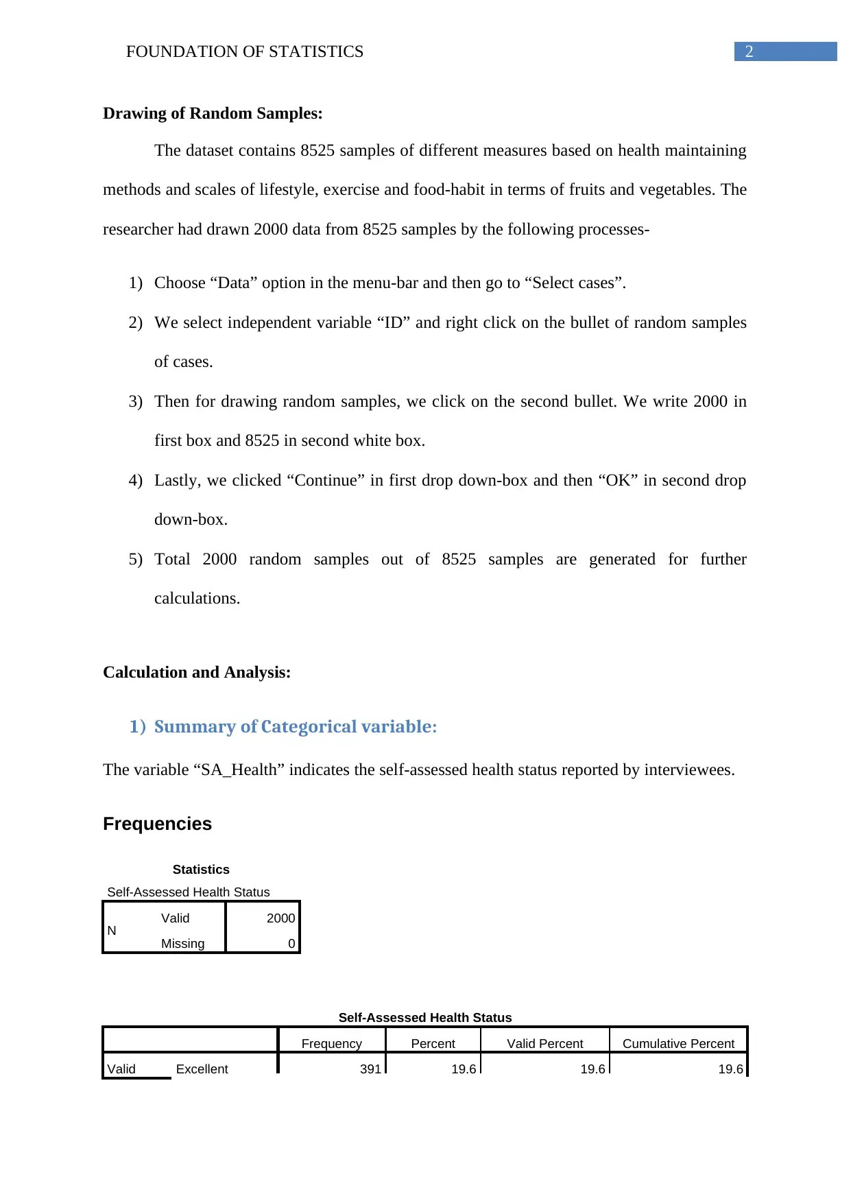
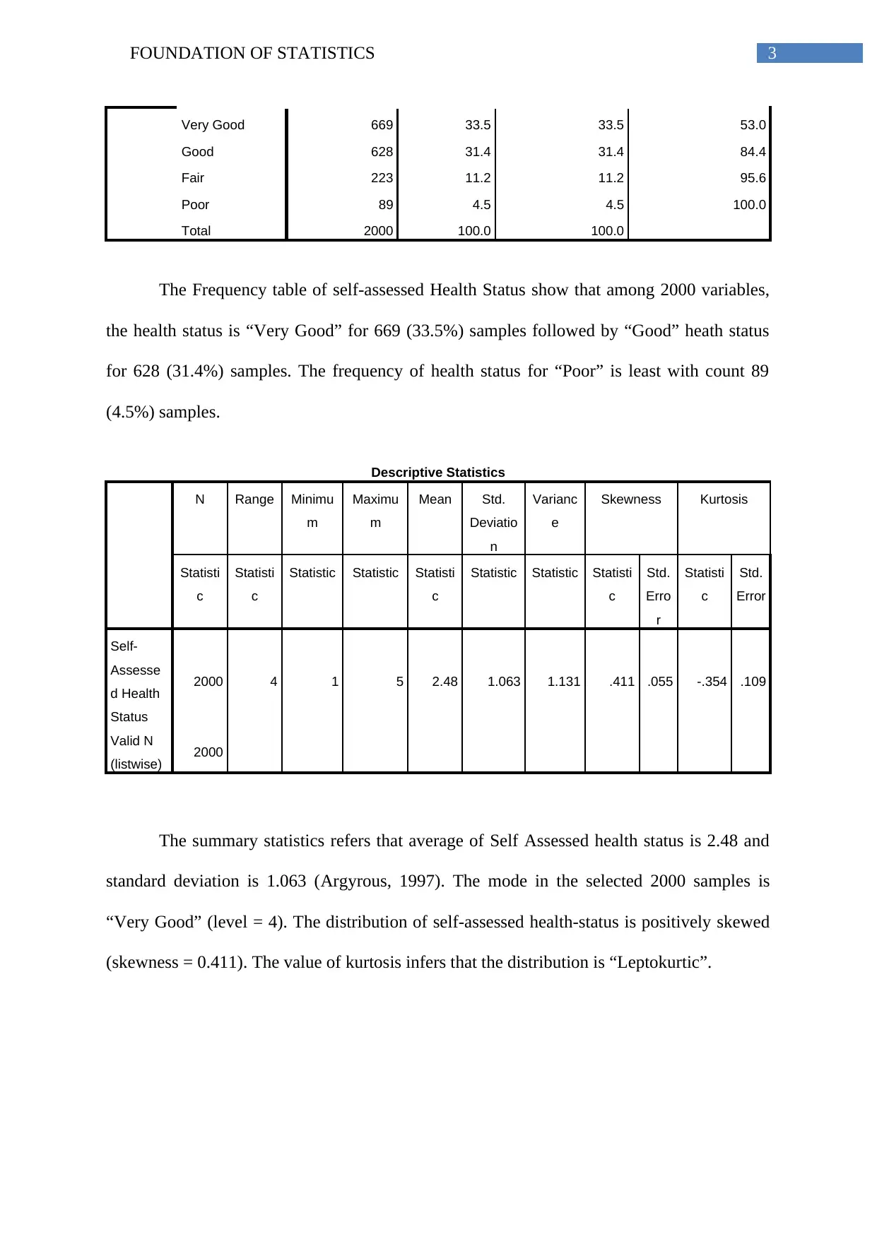
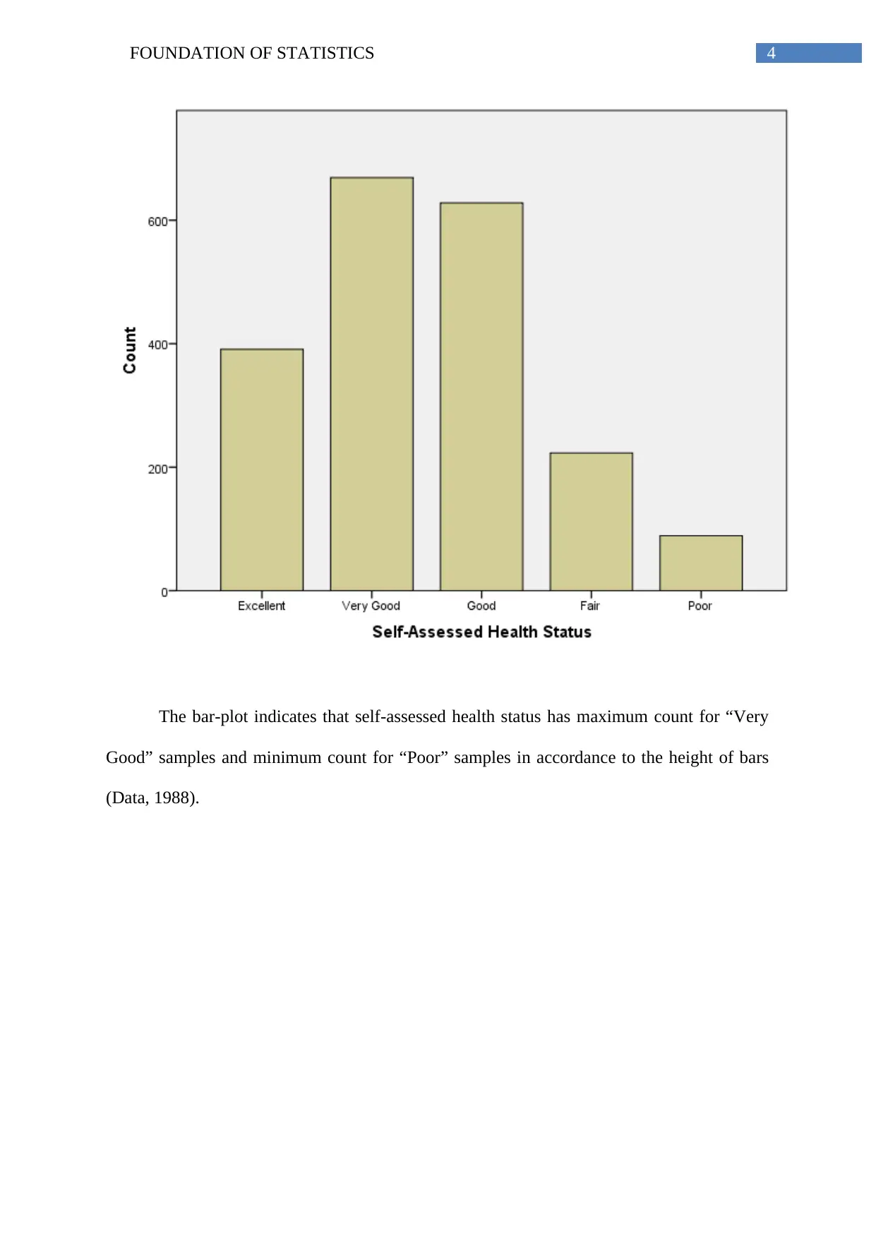
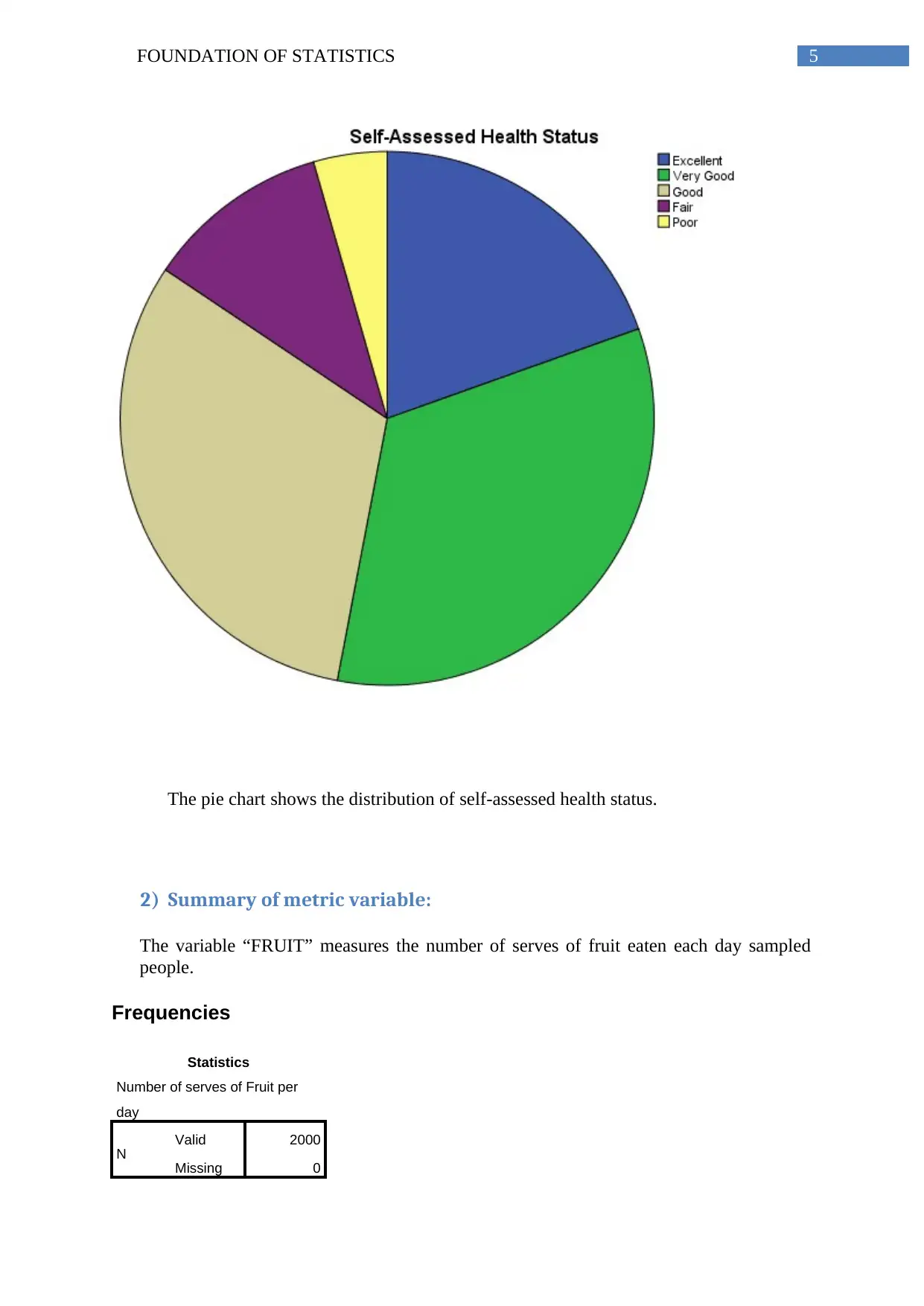
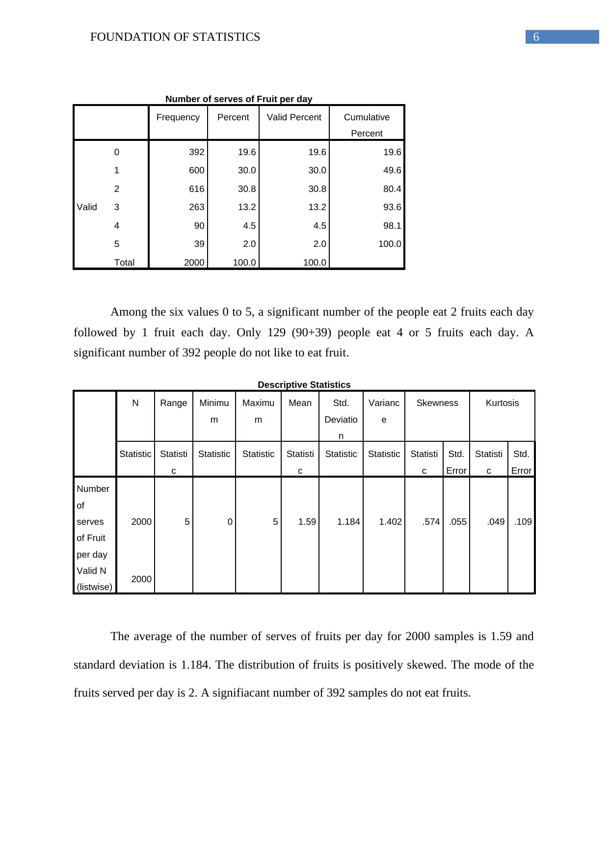
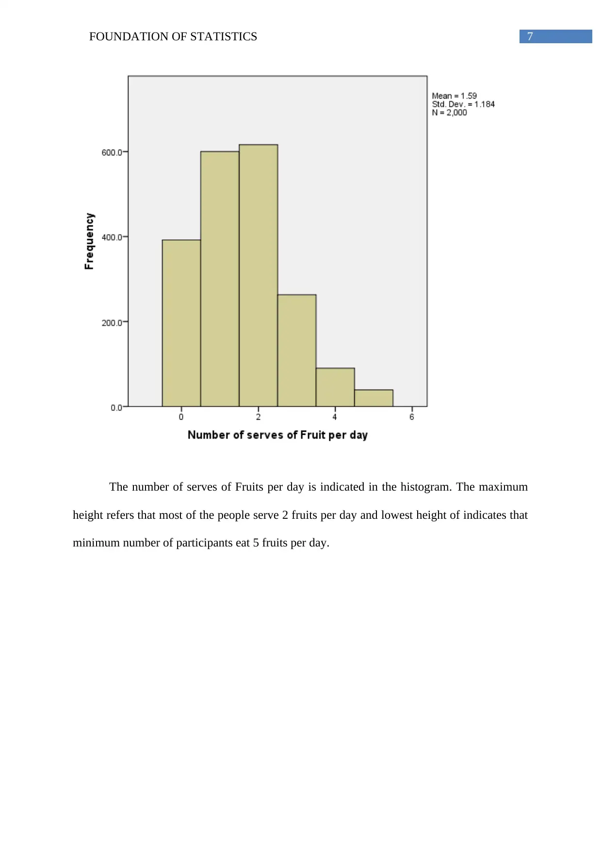
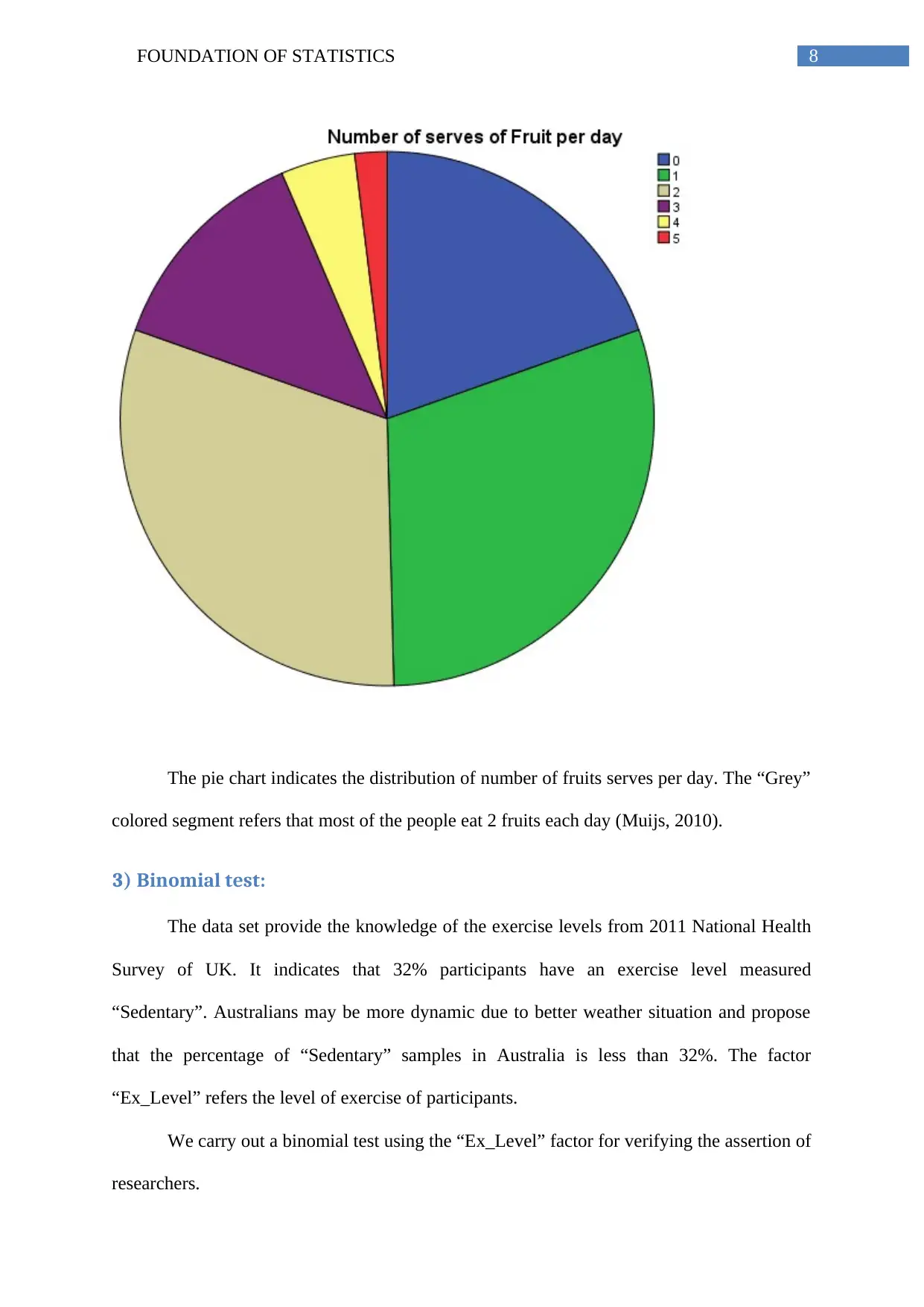
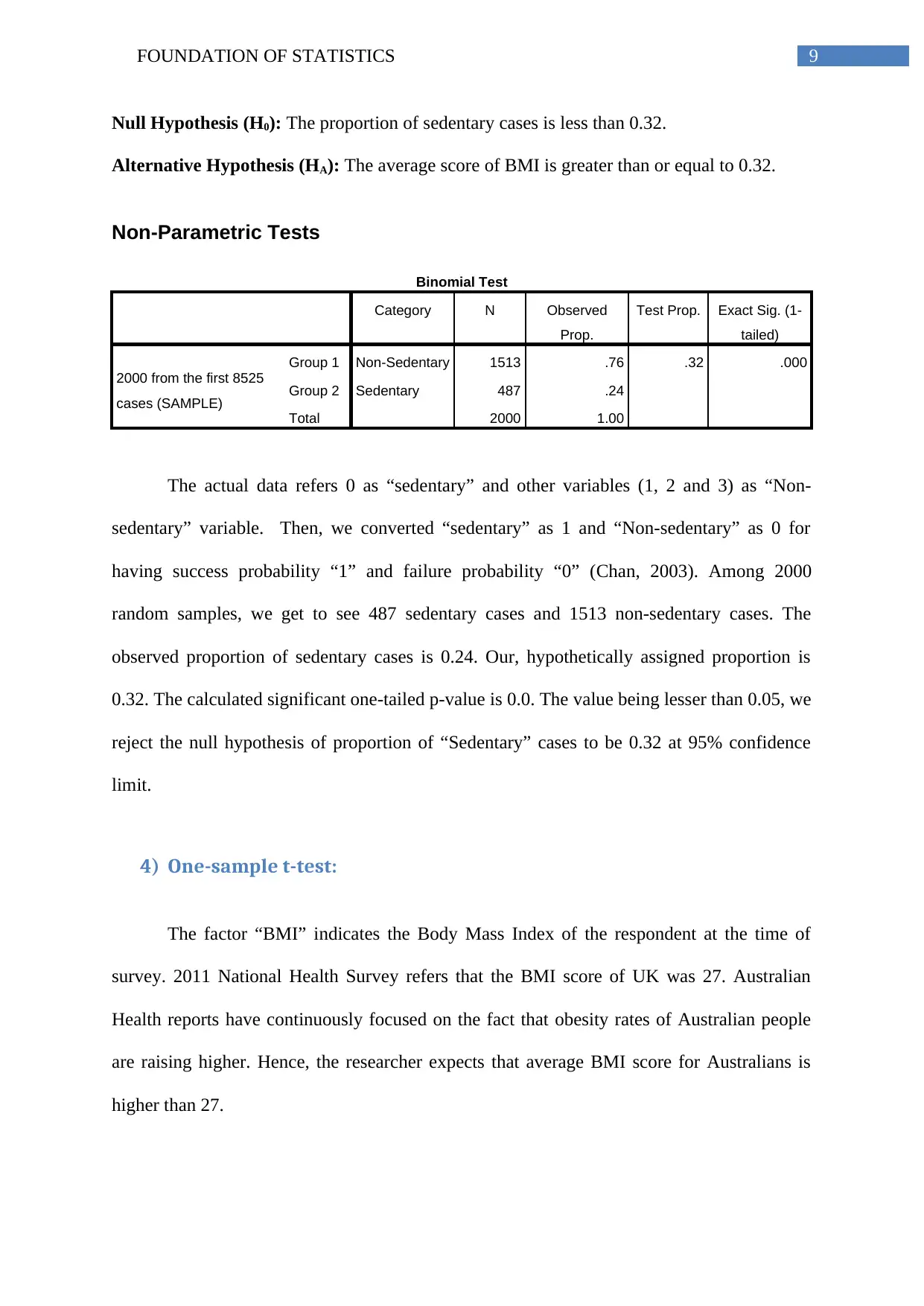
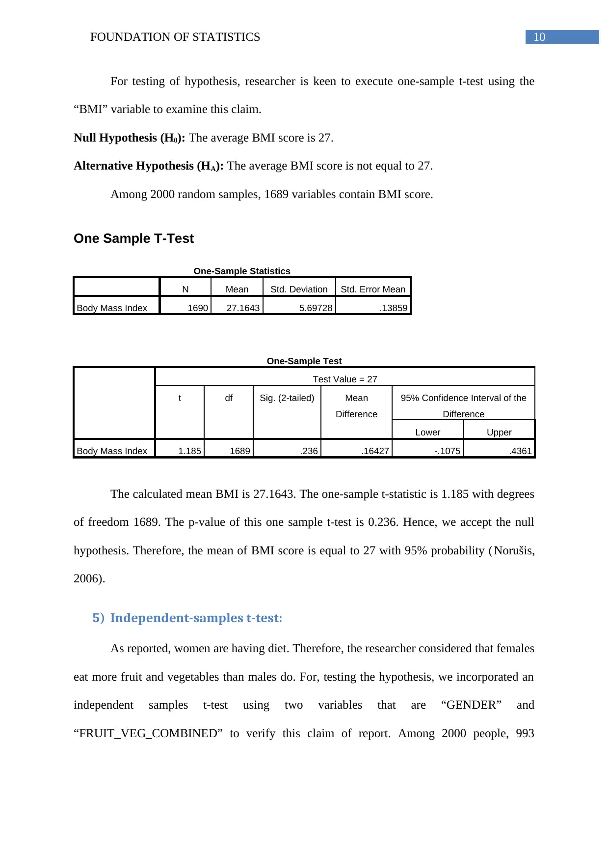
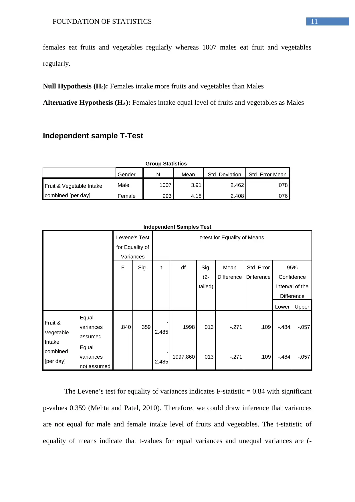
This assignment analyzes a dataset of 8525 samples related to health, lifestyle, exercise, and diet. It begins by drawing 2000 random samples for analysis. The assignment then summarizes categorical variables (self-assessed health status) and metric variables (fruit consumption). Statistical tests, including binomial and one-sample t-tests, are performed to test hypotheses about exercise levels and BMI scores. An independent-samples t-test is used to compare fruit and vegetable intake between genders. The analysis includes frequency tables, descriptive statistics, bar plots, pie charts, and histograms to illustrate the data. The results of each test are interpreted, and conclusions are drawn based on the p-values and confidence intervals, offering insights into the relationships between health, lifestyle, and dietary habits.

Running head: FOUNDATION OF STATISTICS
Foundation of Statistics
Name of the Student:
Name of the University:
Author’s note:

1FOUNDATION OF STATISTICS
Table of Contents
Calculation and Analysis:..........................................................................................................2
1) Summary of Categorical variable:...............................................................................2
2) Summary of metric variable:.......................................................................................5
3) Binomial test:.....................................................................................................................8
4) One-sample t-test:........................................................................................................9
5) Independent-samples t-test:.......................................................................................10
References:...............................................................................................................................12

2FOUNDATION OF STATISTICS
Drawing of Random Samples:
The dataset contains 8525 samples of different measures based on health maintaining
methods and scales of lifestyle, exercise and food-habit in terms of fruits and vegetables. The
researcher had drawn 2000 data from 8525 samples by the following processes-
1) Choose “Data” option in the menu-bar and then go to “Select cases”.
2) We select independent variable “ID” and right click on the bullet of random samples
of cases.
3) Then for drawing random samples, we click on the second bullet. We write 2000 in
first box and 8525 in second white box.
4) Lastly, we clicked “Continue” in first drop down-box and then “OK” in second drop
down-box.
5) Total 2000 random samples out of 8525 samples are generated for further
calculations.
Calculation and Analysis:
1) Summary of Categorical variable:
The variable “SA_Health” indicates the self-assessed health status reported by interviewees.
Frequencies
Statistics
Self-Assessed Health Status
N Valid 2000
Missing 0
Self-Assessed Health Status
Frequency Percent Valid Percent Cumulative Percent
Valid Excellent 391 19.6 19.6 19.6

3FOUNDATION OF STATISTICS
Very Good 669 33.5 33.5 53.0
Good 628 31.4 31.4 84.4
Fair 223 11.2 11.2 95.6
Poor 89 4.5 4.5 100.0
Total 2000 100.0 100.0
The Frequency table of self-assessed Health Status show that among 2000 variables,
the health status is “Very Good” for 669 (33.5%) samples followed by “Good” heath status
for 628 (31.4%) samples. The frequency of health status for “Poor” is least with count 89
(4.5%) samples.
Descriptive Statistics
N Range Minimu
m
Maximu
m
Mean Std.
Deviatio
n
Varianc
e
Skewness Kurtosis
Statisti
c
Statisti
c
Statistic Statistic Statisti
c
Statistic Statistic Statisti
c
Std.
Erro
r
Statisti
c
Std.
Error
Self-
Assesse
d Health
Status
2000 4 1 5 2.48 1.063 1.131 .411 .055 -.354 .109
Valid N
(listwise) 2000
The summary statistics refers that average of Self Assessed health status is 2.48 and
standard deviation is 1.063 (Argyrous, 1997). The mode in the selected 2000 samples is
“Very Good” (level = 4). The distribution of self-assessed health-status is positively skewed
(skewness = 0.411). The value of kurtosis infers that the distribution is “Leptokurtic”.

4FOUNDATION OF STATISTICS
The bar-plot indicates that self-assessed health status has maximum count for “Very
Good” samples and minimum count for “Poor” samples in accordance to the height of bars
(Data, 1988).

5FOUNDATION OF STATISTICS
The pie chart shows the distribution of self-assessed health status.
2) Summary of metric variable:
The variable “FRUIT” measures the number of serves of fruit eaten each day sampled
people.
Frequencies
Statistics
Number of serves of Fruit per
day
N Valid 2000
Missing 0

6FOUNDATION OF STATISTICS
Number of serves of Fruit per day
Frequency Percent Valid Percent Cumulative
Percent
Valid
0 392 19.6 19.6 19.6
1 600 30.0 30.0 49.6
2 616 30.8 30.8 80.4
3 263 13.2 13.2 93.6
4 90 4.5 4.5 98.1
5 39 2.0 2.0 100.0
Total 2000 100.0 100.0
Among the six values 0 to 5, a significant number of the people eat 2 fruits each day
followed by 1 fruit each day. Only 129 (90+39) people eat 4 or 5 fruits each day. A
significant number of 392 people do not like to eat fruit.
Descriptive Statistics
N Range Minimu
m
Maximu
m
Mean Std.
Deviatio
n
Varianc
e
Skewness Kurtosis
Statistic Statisti
c
Statistic Statistic Statisti
c
Statistic Statistic Statisti
c
Std.
Error
Statisti
c
Std.
Error
Number
of
serves
of Fruit
per day
2000 5 0 5 1.59 1.184 1.402 .574 .055 .049 .109
Valid N
(listwise) 2000
The average of the number of serves of fruits per day for 2000 samples is 1.59 and
standard deviation is 1.184. The distribution of fruits is positively skewed. The mode of the
fruits served per day is 2. A signifiacant number of 392 samples do not eat fruits.

7FOUNDATION OF STATISTICS
The number of serves of Fruits per day is indicated in the histogram. The maximum
height refers that most of the people serve 2 fruits per day and lowest height of indicates that
minimum number of participants eat 5 fruits per day.

8FOUNDATION OF STATISTICS
The pie chart indicates the distribution of number of fruits serves per day. The “Grey”
colored segment refers that most of the people eat 2 fruits each day (Muijs, 2010).
3) Binomial test:
The data set provide the knowledge of the exercise levels from 2011 National Health
Survey of UK. It indicates that 32% participants have an exercise level measured
“Sedentary”. Australians may be more dynamic due to better weather situation and propose
that the percentage of “Sedentary” samples in Australia is less than 32%. The factor
“Ex_Level” refers the level of exercise of participants.
We carry out a binomial test using the “Ex_Level” factor for verifying the assertion of
researchers.

9FOUNDATION OF STATISTICS
Null Hypothesis (H0): The proportion of sedentary cases is less than 0.32.
Alternative Hypothesis (HA): The average score of BMI is greater than or equal to 0.32.
Non-Parametric Tests
Binomial Test
Category N Observed
Prop.
Test Prop. Exact Sig. (1-
tailed)
2000 from the first 8525
cases (SAMPLE)
Group 1 Non-Sedentary 1513 .76 .32 .000
Group 2 Sedentary 487 .24
Total 2000 1.00
The actual data refers 0 as “sedentary” and other variables (1, 2 and 3) as “Non-
sedentary” variable. Then, we converted “sedentary” as 1 and “Non-sedentary” as 0 for
having success probability “1” and failure probability “0” (Chan, 2003). Among 2000
random samples, we get to see 487 sedentary cases and 1513 non-sedentary cases. The
observed proportion of sedentary cases is 0.24. Our, hypothetically assigned proportion is
0.32. The calculated significant one-tailed p-value is 0.0. The value being lesser than 0.05, we
reject the null hypothesis of proportion of “Sedentary” cases to be 0.32 at 95% confidence
limit.
4) One-sample t-test:
The factor “BMI” indicates the Body Mass Index of the respondent at the time of
survey. 2011 National Health Survey refers that the BMI score of UK was 27. Australian
Health reports have continuously focused on the fact that obesity rates of Australian people
are raising higher. Hence, the researcher expects that average BMI score for Australians is
higher than 27.

10FOUNDATION OF STATISTICS
For testing of hypothesis, researcher is keen to execute one-sample t-test using the
“BMI” variable to examine this claim.
Null Hypothesis (H0): The average BMI score is 27.
Alternative Hypothesis (HA): The average BMI score is not equal to 27.
Among 2000 random samples, 1689 variables contain BMI score.
One Sample T-Test
One-Sample Statistics
N Mean Std. Deviation Std. Error Mean
Body Mass Index 1690 27.1643 5.69728 .13859
One-Sample Test
Test Value = 27
t df Sig. (2-tailed) Mean
Difference
95% Confidence Interval of the
Difference
Lower Upper
Body Mass Index 1.185 1689 .236 .16427 -.1075 .4361
The calculated mean BMI is 27.1643. The one-sample t-statistic is 1.185 with degrees
of freedom 1689. The p-value of this one sample t-test is 0.236. Hence, we accept the null
hypothesis. Therefore, the mean of BMI score is equal to 27 with 95% probability (Norušis,
2006).
5) Independent-samples t-test:
As reported, women are having diet. Therefore, the researcher considered that females
eat more fruit and vegetables than males do. For, testing the hypothesis, we incorporated an
independent samples t-test using two variables that are “GENDER” and
“FRUIT_VEG_COMBINED” to verify this claim of report. Among 2000 people, 993

11FOUNDATION OF STATISTICS
females eat fruits and vegetables regularly whereas 1007 males eat fruit and vegetables
regularly.
Null Hypothesis (H0): Females intake more fruits and vegetables than Males
Alternative Hypothesis (HA): Females intake equal level of fruits and vegetables as Males
Independent sample T-Test
Group Statistics
Gender N Mean Std. Deviation Std. Error Mean
Fruit & Vegetable Intake
combined [per day]
Male 1007 3.91 2.462 .078
Female 993 4.18 2.408 .076
Independent Samples Test
Levene's Test
for Equality of
Variances
t-test for Equality of Means
F Sig. t df Sig.
(2-
tailed)
Mean
Difference
Std. Error
Difference
95%
Confidence
Interval of the
Difference
Lower Upper
Fruit &
Vegetable
Intake
combined
[per day]
Equal
variances
assumed
.840 .359 -
2.485 1998 .013 -.271 .109 -.484 -.057
Equal
variances
not assumed
-
2.485 1997.860 .013 -.271 .109 -.484 -.057
The Levene’s test for equality of variances indicates F-statistic = 0.84 with significant
p-values 0.359 (Mehta and Patel, 2010). Therefore, we could draw inference that variances
are not equal for male and female intake level of fruits and vegetables. The t-statistic of
equality of means indicate that t-values for equal variances and unequal variances are (-