Frequency Response & Bode Plots Analysis - Electrical Engineering
VerifiedAdded on 2023/04/19
|6
|618
|113
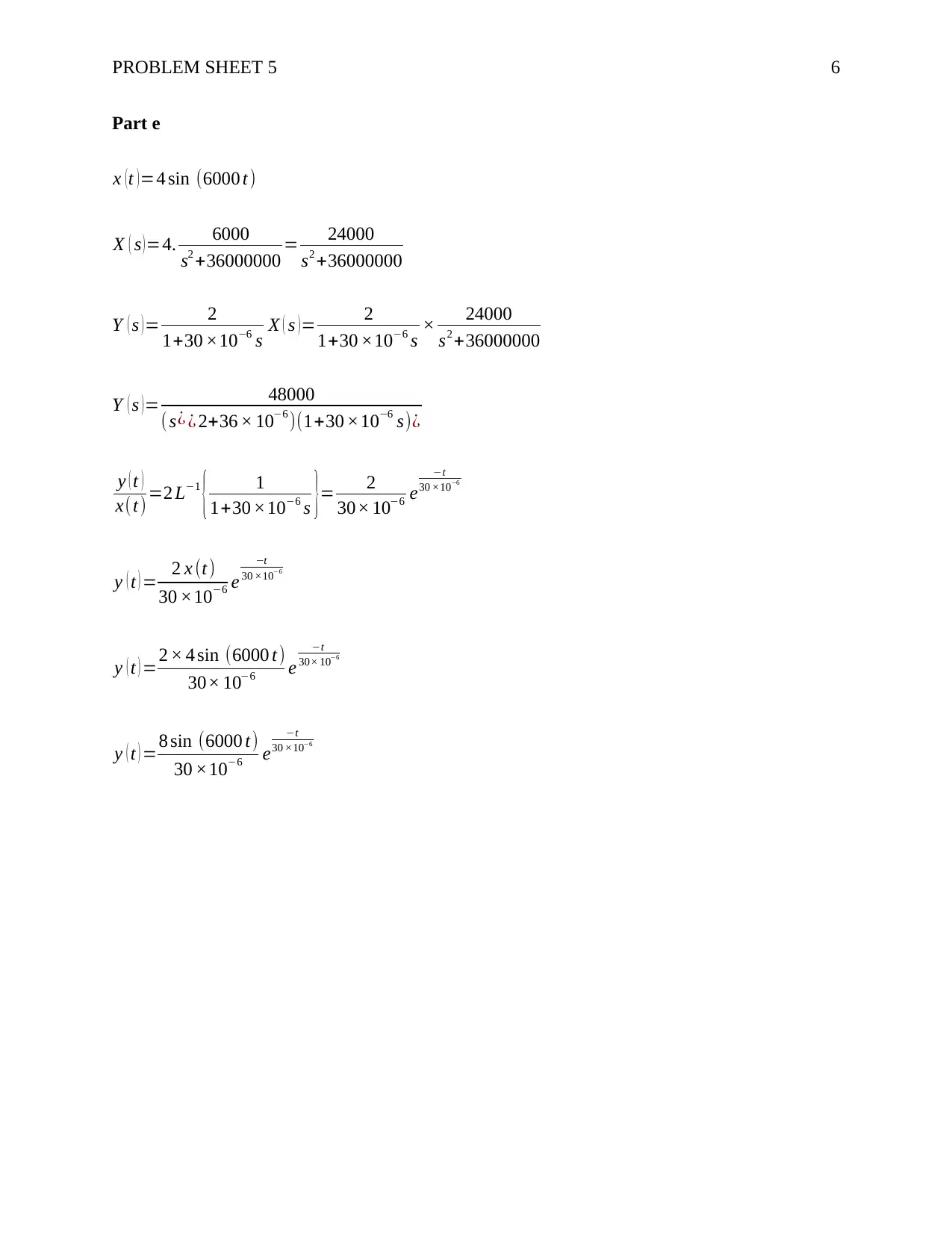
Homework Assignment
AI Summary
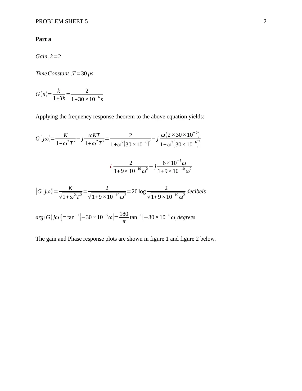
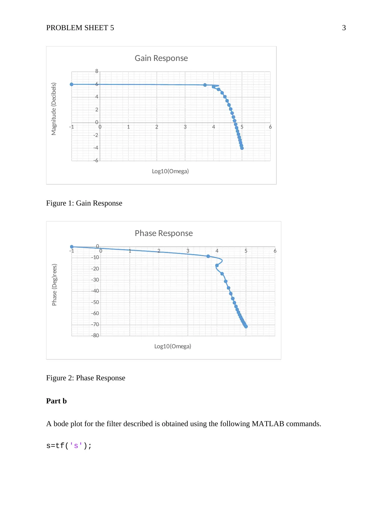
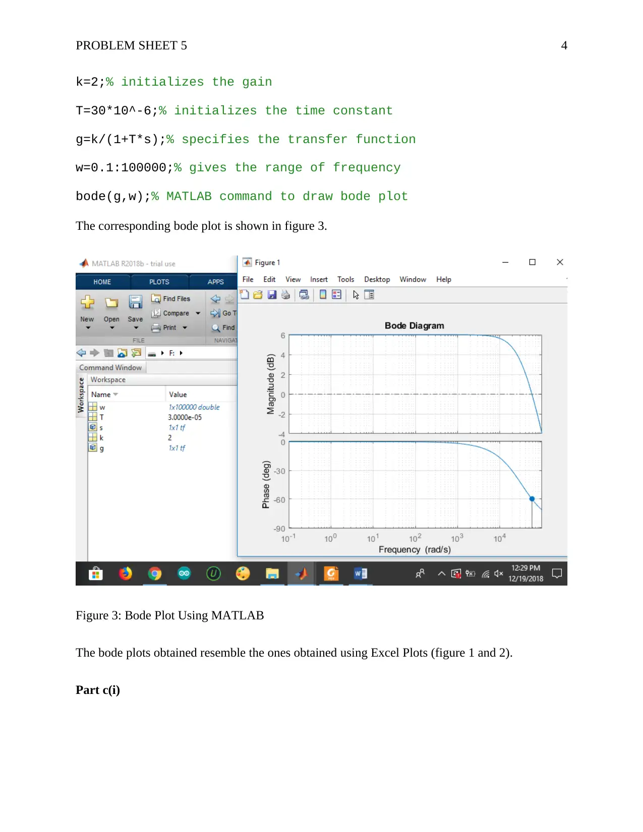
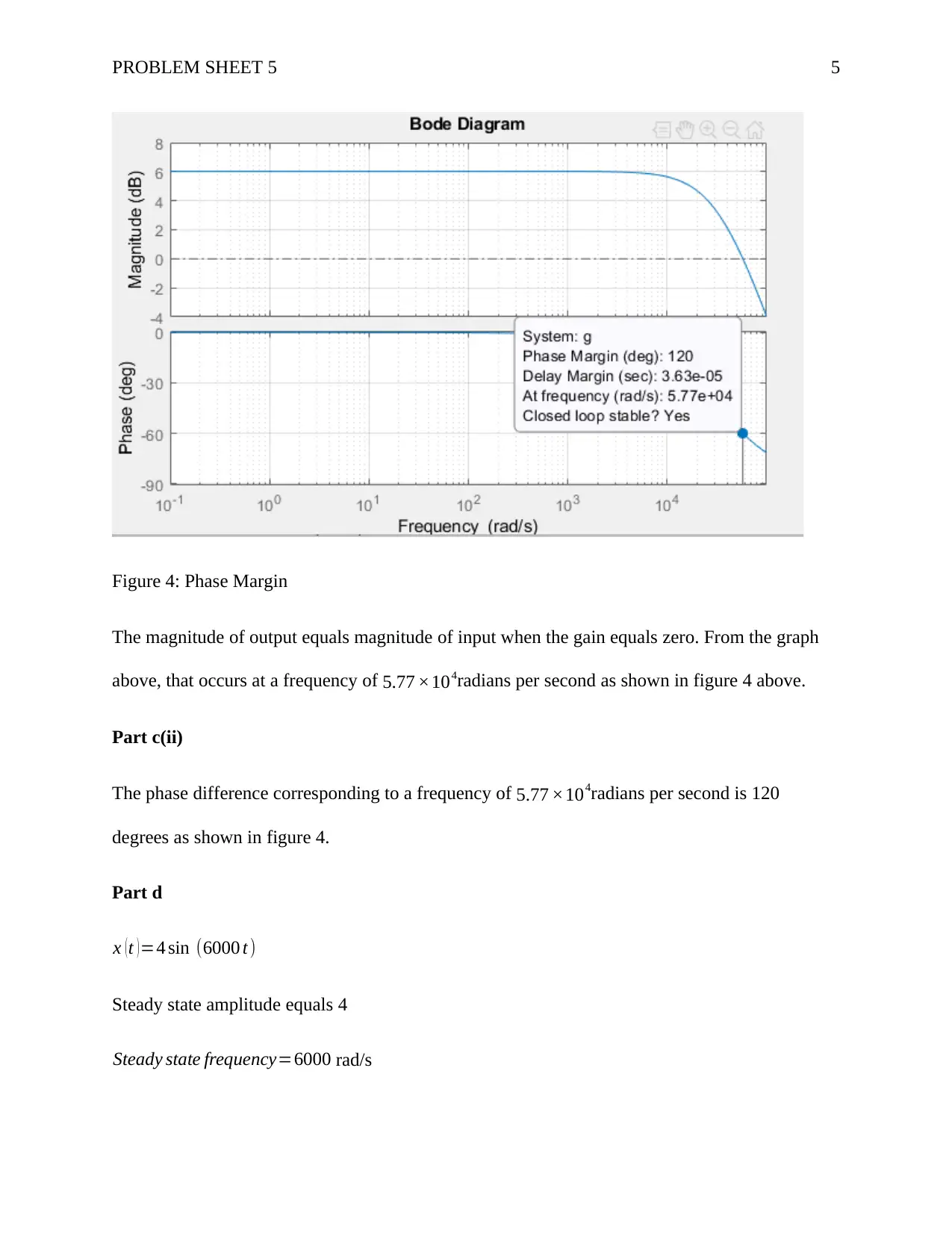
This assignment solution addresses Problem Sheet 5, focusing on the frequency response of a first-order filter with a gain of 2 and a time constant of 30μs. The solution involves using the Frequency Response Theorem to compute the gain and phase response, generating Bode plots using both Excel and MATLAB, determining the frequency at which the output magnitude equals the input magnitude, and calculating the corresponding phase difference. Additionally, the response to a sinusoidal input signal is analyzed, and the steady-state amplitude and frequency are determined. The solution includes MATLAB code, plots, and detailed mathematical derivations, providing a comprehensive analysis of the filter's behavior. Desklib provides a platform for students to access such solved assignments and study materials.

1 out of 6
Related Documents


Your All-in-One AI-Powered Toolkit for Academic Success.
+13062052269
info@desklib.com
Available 24*7 on WhatsApp / Email
![[object Object]](/_next/static/media/star-bottom.7253800d.svg)
Copyright © 2020–2026 A2Z Services. All Rights Reserved. Developed and managed by ZUCOL.