Major Assignment: MAF101 Fundamentals of Finance - Trimester 1, 2019

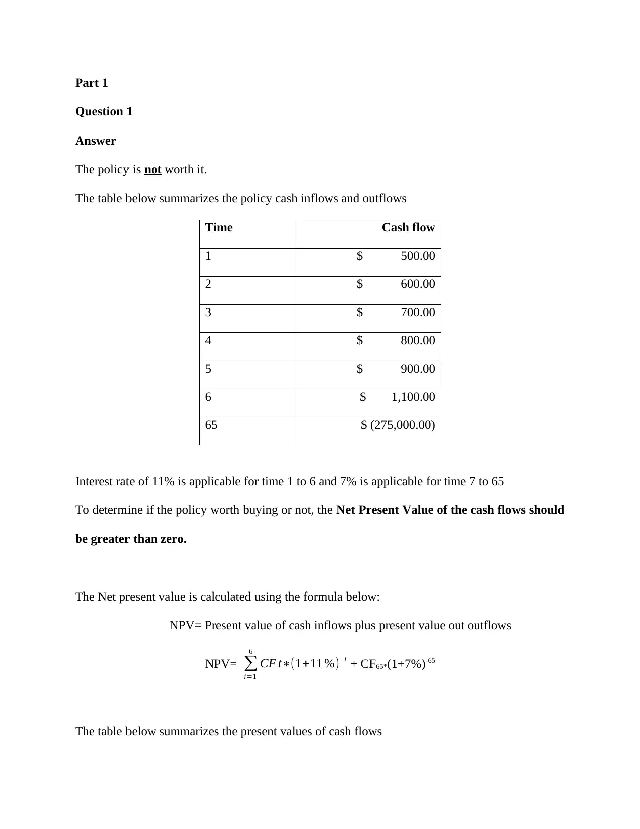
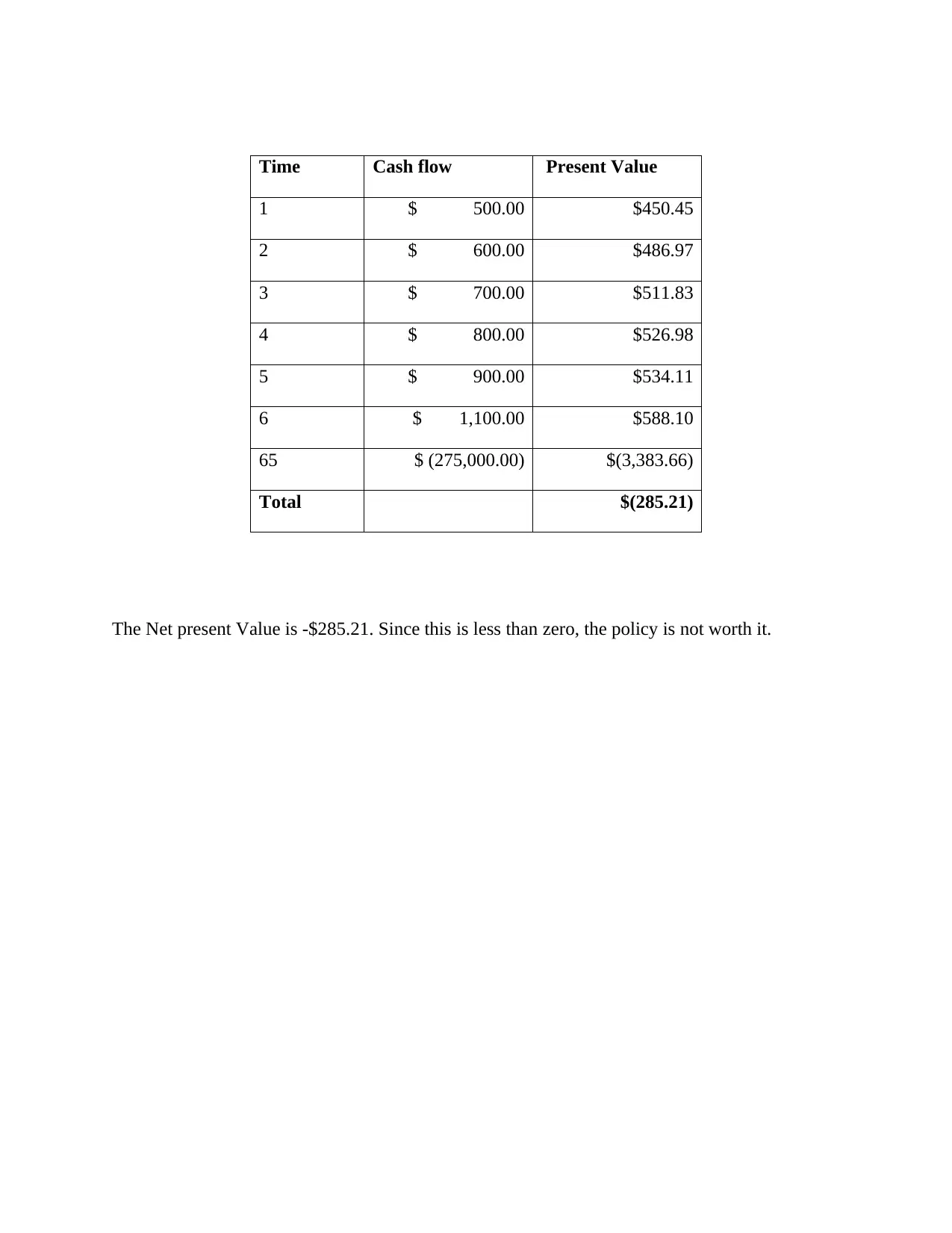
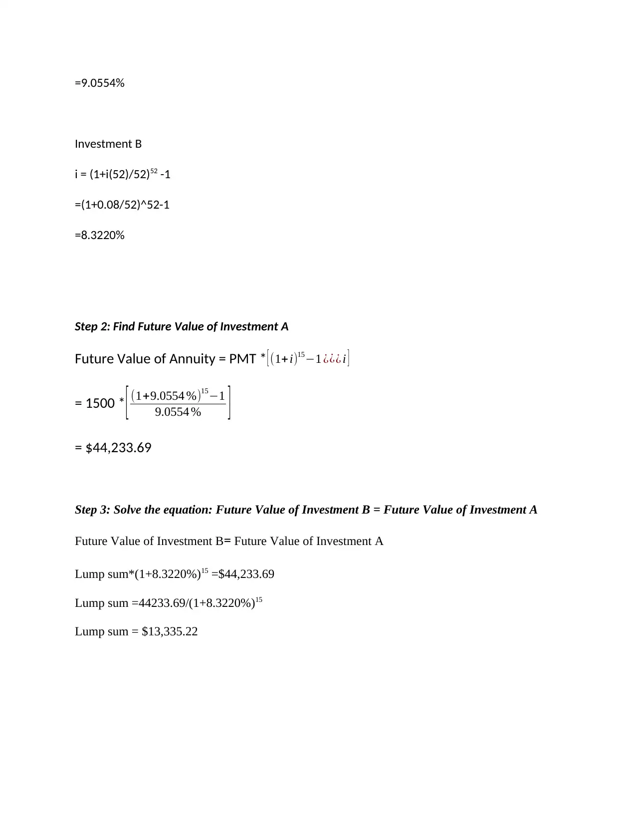
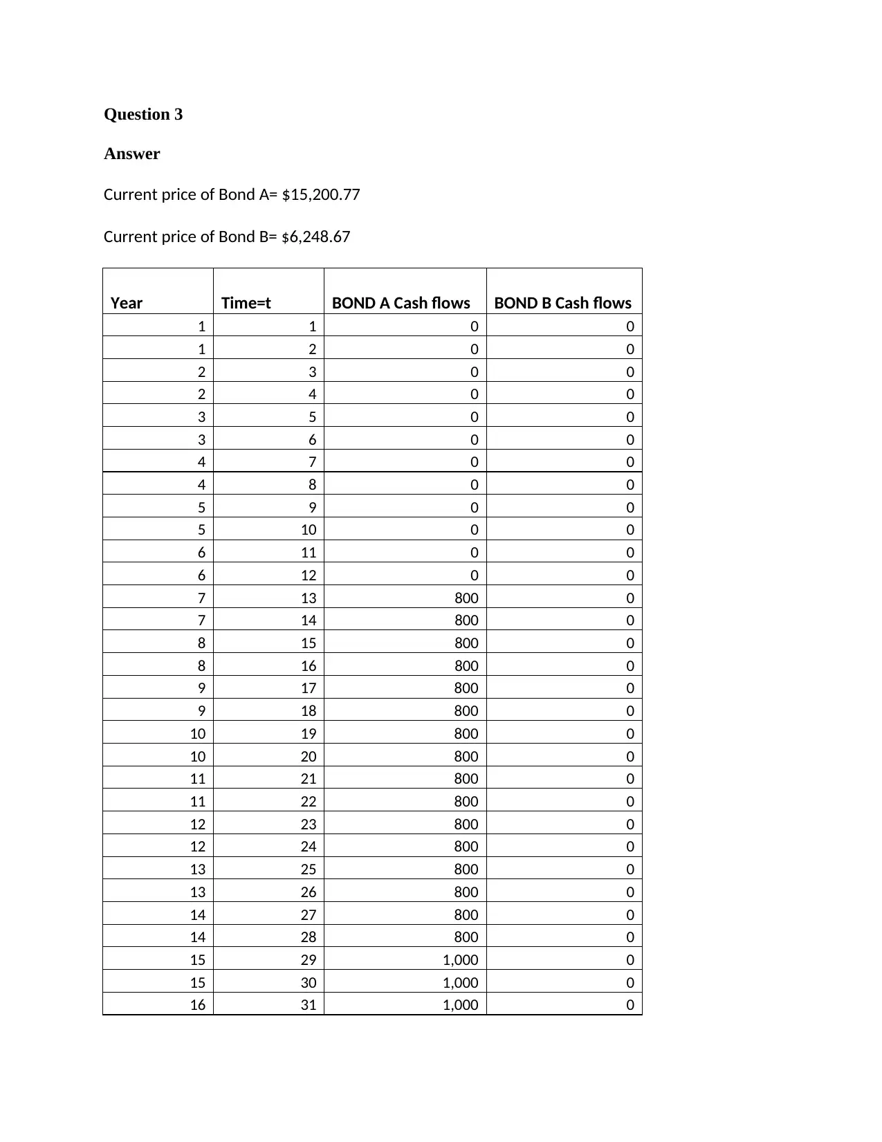
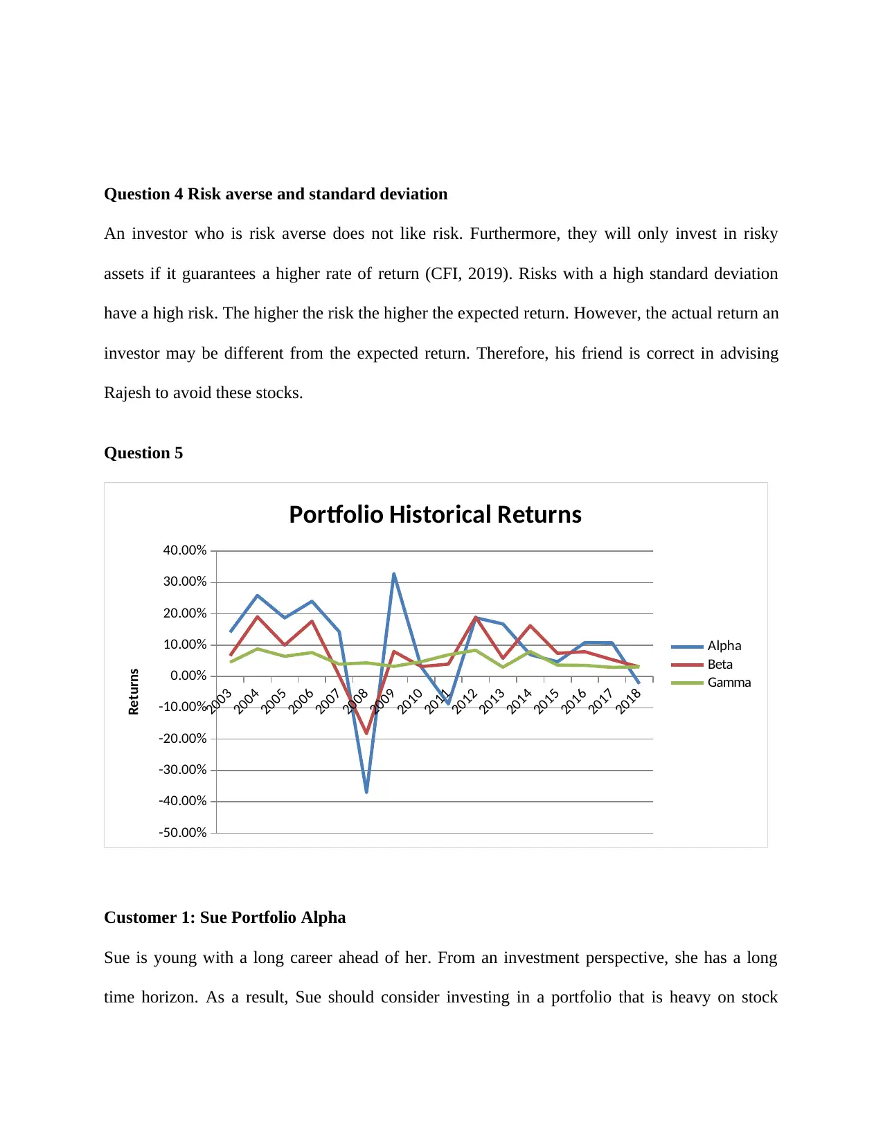
This assignment solution for MAF101, Fundamentals of Finance, covers several key financial concepts. Part 1 includes calculations for net present value, lump sum investments, bond pricing, and share valuation using the dividend growth model. Part 2 focuses on portfolio analysis, exploring the returns and risks associated with different investment strategies. It analyzes portfolio alpha, beta, and gamma, using historical data to assess risk and return profiles. The solution also addresses risk management principles, including diversifiable and non-diversifiable risks, the use of beta and standard deviation, and the implications of risk aversion. Finally, the assignment provides investment recommendations for different customer profiles based on their time horizons and risk tolerance.

Part 1
Question 1
Answer
The policy is not worth it.
The table below summarizes the policy cash inflows and outflows
Time Cash flow
1 $ 500.00
2 $ 600.00
3 $ 700.00
4 $ 800.00
5 $ 900.00
6 $ 1,100.00
65 $ (275,000.00)
Interest rate of 11% is applicable for time 1 to 6 and 7% is applicable for time 7 to 65
To determine if the policy worth buying or not, the Net Present Value of the cash flows should
be greater than zero.
The Net present value is calculated using the formula below:
NPV= Present value of cash inflows plus present value out outflows
NPV= ∑
i=1
6
CF t∗(1+11 %)−t + CF65*(1+7%)-65
The table below summarizes the present values of cash flows

Time Cash flow Present Value
1 $ 500.00 $450.45
2 $ 600.00 $486.97
3 $ 700.00 $511.83
4 $ 800.00 $526.98
5 $ 900.00 $534.11
6 $ 1,100.00 $588.10
65 $ (275,000.00) $(3,383.66)
Total $(285.21)
The Net present Value is -$285.21. Since this is less than zero, the policy is not worth it.

Question 2
Answer
A lump sum of $13,335.22 should be invested in B today.
To find the lump sum, we need to solve the equation:
Future Value of Investment B = Future Value of Investment A
Investment A
n =15-year annuity
PMT= $1,500
i(12) =interest rate of 8.7 percent compounded monthly
Investment B
n =15-year Lump sum
i(52) = interest 8 percent compounded weekly
Step 1: Find annual effective rate of interest, i for both investments
1+i = (1+ j
n)n (Madura, 2009)
Where i is the effective rate and j is the nominal rate of interest
Investment A
i = (1+i(12)/12)12 -1
=(1+0.087/12)^12-1

=9.0554%
Investment B
i = (1+i(52)/52)52 -1
=(1+0.08/52)^52-1
=8.3220%
Step 2: Find Future Value of Investment A
Future Value of Annuity = PMT * [ (1+ i)15−1 ¿¿¿ i ]
= 1500 * [ (1+9.0554 %)15−1
9.0554 % ]
= $44,233.69
Step 3: Solve the equation: Future Value of Investment B = Future Value of Investment A
Future Value of Investment B= Future Value of Investment A
Lump sum*(1+8.3220%)15 =$44,233.69
Lump sum =44233.69/(1+8.3220%)15
Lump sum = $13,335.22

Question 3
Answer
Current price of Bond A= $15,200.77
Current price of Bond B= $6,248.67
Year Time=t BOND A Cash flows BOND B Cash flows
1 1 0 0
1 2 0 0
2 3 0 0
2 4 0 0
3 5 0 0
3 6 0 0
4 7 0 0
4 8 0 0
5 9 0 0
5 10 0 0
6 11 0 0
6 12 0 0
7 13 800 0
7 14 800 0
8 15 800 0
8 16 800 0
9 17 800 0
9 18 800 0
10 19 800 0
10 20 800 0
11 21 800 0
11 22 800 0
12 23 800 0
12 24 800 0
13 25 800 0
13 26 800 0
14 27 800 0
14 28 800 0
15 29 1,000 0
15 30 1,000 0
16 31 1,000 0

16 32 1,000 0
17 33 1,000 0
17 34 1,000 0
18 35 1,000 0
18 36 1,000 0
19 37 1,000 0
19 38 1,000 0
20 39 1,000 0
20 40 31,000 30,000
Current price of Bond A
Face value = $30,000
n= 20 years.
PMT= $800 every six months for eight years after year 6, and finally pays $1,000 every six
months over the last six year
i(2)=8 percent compounded semiannually
Effective semiannual interest rate = i(2)/2= 4%
PV= 800 *[ 1−(1+4 %)−16 ¿¿¿ i ]∗(1+ 4 %)−12+ 1,000 * [ 1−(1+4 %)−12 ¿ ¿¿ i ]∗(1+ 4 % )−28+ ¿
30,000 * (1+4%)-40
= $15,200.77
Current price of Bond B
Face value =$30,000
n= 20 years
Nill coupon payments

PV =30,000*(1+4%)-20
= $6,248.67

Question 4
The price of share can be determined using the Dividend growth model (Ro, 2015)
Present Value = D1/(k- g)
Where D1 = dividend paid for period, k = required return and g = growth factor (CF1, 2019).
D1= $1.95
K=11%
g=6%
Current price
PV = 1.95/(11%-6%)
=$39
Price in 3 years
=P0*(1+11%)3
=39*(1+11%)^3
=$53.34

Part 2
Question 1
PORTFOLIO ALPHA: 80% shares; 10% property; 10% cash.
Expected Returns =80%*Shares(t)+ 10%*Property(t) + 10%*cash(t)
PORTFOLIO BETA: 50% bonds; 10% shares; 40% property
Expected Returns =50%*bonds(t)+ 10%*shares(t) + 10%*property(t)
PORTFOLIO GAMMA: 50% cash; 40% bonds; 10% property
Expected Returns =50%*cash(t)+ 40%*bonds(t) + 10%*property(t)
a) Historical returns for the years between 2003 and 2018
Year Shares Propert
y Bonds Cash Alpha Beta Gamma
2003 15.90% 8.80% 3.00% 4.90% 14.09% 6.61% 4.53%
2004 27.60% 32.00% 7.00% 5.60% 25.84% 19.06% 8.80%
2005 21.10% 12.50% 5.80% 5.70% 18.70% 10.01% 6.42%
2006 25.00% 34.00% 3.10% 6.00% 24.00% 17.65% 7.64%
2007 18.00% -8.40% 3.50% 6.70% 14.23% 0.19% 3.91%
2008 -
40.40% -54.00% 14.90% 7.60% -36.96% -18.19% 4.36%
2009 39.60% 7.90% 1.70% 3.50% 32.82% 7.97% 3.22%
2010 3.30% -0.40% 6.00% 4.70% 3.07% 3.17% 4.71%
2011 -
11.40% -1.50% 11.40% 5.00% -8.77% 3.96% 6.91%
2012 18.80% 33.00% 7.70% 4.00% 18.74% 18.93% 8.38%
2013 19.70% 7.10% 2.00% 2.90% 16.76% 5.81% 2.96%
2014 5.00% 27.00% 9.80% 2.70% 6.97% 16.20% 7.97%
2015 3.80% 14.30% 2.60% 2.30% 4.70% 7.40% 3.62%
2016 11.60% 13.20% 2.90% 2.10% 10.81% 7.89% 3.53%
2017 12.50% 5.70% 3.70% 1.70% 10.74% 5.38% 2.90%
2018 -3.50% 2.90% 4.50% 1.90% -2.32% 3.06% 3.04%
b)

Year Shares Property Bonds Cash Alpha Beta Gamm
a
2003 15.90% 8.80% 3.00% 4.90% 14.09% 6.61% 4.53%
2004 27.60% 32.00% 7.00% 5.60% 25.84% 19.06% 8.80%
2005 21.10% 12.50% 5.80% 5.70% 18.70% 10.01% 6.42%
2006 25.00% 34.00% 3.10% 6.00% 24.00% 17.65% 7.64%
2007 18.00% -8.40% 3.50% 6.70% 14.23% 0.19% 3.91%
2008 -40.40% -54.00% 14.90% 7.60% -36.96% -18.19% 4.36%
2009 39.60% 7.90% 1.70% 3.50% 32.82% 7.97% 3.22%
2010 3.30% -0.40% 6.00% 4.70% 3.07% 3.17% 4.71%
2011 -11.40% -1.50% 11.40% 5.00% -8.77% 3.96% 6.91%
2012 18.80% 33.00% 7.70% 4.00% 18.74% 18.93% 8.38%
2013 19.70% 7.10% 2.00% 2.90% 16.76% 5.81% 2.96%
2014 5.00% 27.00% 9.80% 2.70% 6.97% 16.20% 7.97%
2015 3.80% 14.30% 2.60% 2.30% 4.70% 7.40% 3.62%
2016 11.60% 13.20% 2.90% 2.10% 10.81% 7.89% 3.53%
2017 12.50% 5.70% 3.70% 1.70% 10.74% 5.38% 2.90%
2018 -3.50% 2.90% 4.50% 1.90% -2.32% 3.06% 3.04%
E (R) 10.41% 8.38% 5.60% 4.21% 9.59% 7.19% 5.18%
Risk 0.1844 0.2102 0.0375 0.0184 0.1632 0.0902 0.0213

Question 2
Diversifiable risk (also known as unsystematic risk) is unique to that asset. It can be eliminated
by investing in a portfolio with different assets whose returns are not correlated. Non-
diversifiable risk (also known as market or systematic risk) affects the entire market (Mitchell &
Mulherin, 1996). As a result, it cannot be diversified away by investing in multiple assets (Ben-
Horim & Levy, 1980).
Control of the risks
Indeed investors can control both the level of unsystematic risk and systematic risk in a portfolio.
For unsystematic, this is through diversification. For systematic, diversification will not work,
though options like hedging may control the risk (The Balance, 2018). However, controlling the
level of risk will be a costly effect on the portfolio’s estimated returns- the higher the risk the
higher the expected return (Inside Business, 2012).
Question 3- Beta and Standard deviation
The beta coefficient is a measure of a stock’s market risk, or the extent to which the returns on a
given stock move with the stock market. It measures the individual stocks volatility in
comparison to the entire market (Rosenberg & Guy, 1995). On the other hand, the standard
deviation measures the stock’s individual risk. Systematic risk cannot be removed no matter how
much an investor diversifies their assets. Therefore, using beta as a measure of risk is more
appropriate for a well-diversified as it takes market risk into consideration (Rosenberg & Guy,
1995).

Question 4 Risk averse and standard deviation
An investor who is risk averse does not like risk. Furthermore, they will only invest in risky
assets if it guarantees a higher rate of return (CFI, 2019). Risks with a high standard deviation
have a high risk. The higher the risk the higher the expected return. However, the actual return an
investor may be different from the expected return. Therefore, his friend is correct in advising
Rajesh to avoid these stocks.
Question 5
2003
2004
2005
2006
2007
2008
2009
2010
2011
2012
2013
2014
2015
2016
2017
2018
-50.00%
-40.00%
-30.00%
-20.00%
-10.00%
0.00%
10.00%
20.00%
30.00%
40.00%
Portfolio Historical Returns
Alpha
Beta
Gamma
Returns
Customer 1: Sue Portfolio Alpha
Sue is young with a long career ahead of her. From an investment perspective, she has a long
time horizon. As a result, Sue should consider investing in a portfolio that is heavy on stock

(McMillan, 2017). This is because stocks usually outperform other less risky assets like bonds in
the long term (Fama, 1970). Even at times when the returns are really low, Sue will still have
time to recoup losses. In this scenario, the alpha portfolio is the best option as it is heavily
weighted with stock. Furthermore, from the graph we observe that it provides the highest average
return in the long run despite the high volatility.
Customer 2- John and Karen (a couple)
John and Karen are both middle aged with high income. Furthermore, they plan to retire in 10
years. From an investment perspective, they have a medium to short time horizon. Therefore, For
this couple we propose that the invest in the Beta portfolio as it provides as it is less risky with
50% invested in bonds, but still allows the couple to get higher returns over the ten year period
from the property investment.
Customer 3- Rajesh
Rajesh is about to retire in 1.5 years. From an investment perspective, he has a short time horizon
and is possibly risk averse. As a result, he should consider investing in a portfolio that is less
risky with assets like bonds and cash –in this case the gamma portfolio is the best option since
90% is invested in bonds and cash. Furthermore, the portfolio returns are stable and it provides
the highest liquidity to Rajesh.

References
Ben-Horim, M. & Levy, H., 1980. Total Risk, Diversifiable Risk and Nondiversifiable Risk: A Pedagogic
Note.. Journal of Financial and Quantitative Analysis, 15(2)(doi:10.2307/2330346), pp. 289-297.
CF1, 2019. What is the Gordon Growth Model?. [Online]
Available at: https://corporatefinanceinstitute.com/resources/knowledge/valuation/gordon-growth-
model/
CFI, 2019. What is Risk Averse?. [Online]
Available at: https://corporatefinanceinstitute.com/resources/knowledge/finance/risk-averse-
definition/
Dhaval, S., 2018. Meaning and Type of Dividend Policies. [Online]
Available at: http://www.businessmanagementideas.com/financial-management/dividends/meaning-
and-types-of-dividend-policy-financial-management/3968
Ehrhardt, M. & Brigham, E., 2003. Corporate Finance: A Focused Approach. s.l.:Thomson/South-Western.
Fama, E., 1970. Efficient capital markets: A review of theory and empirical. The Journal of Finance, pp.
383-417.
Inside Business, 2012. The higher the risk, the greater the return. [Online]
Available at: https://pilotonline.com/inside-business/news/columns/article_2b3a069d-57c3-5d16-801e-
8d1698277211.html
Madura, J., 2009. Financial Markets and Institutions. Manson: South-Western Cengage Learning.
McMillan, B., 2017. The Importance Of Time Horizons For Investing (And Beyond). [Online]
Available at: https://www.forbes.com/sites/bradmcmillan/2017/06/27/the-importance-of-time-
horizons-for-investing-and-beyond/#77d06ef92b3d
Mitchell, M. L. & Mulherin, H., 1996. The Impact Of Industry Shocks On Takeover And Restructuring
Activity. Journal of Financial Economics 41, pp. 193-229.
Ro, S., 2015. Goldman Sachs eplains the 'return on equity' formula that every CFA test taker must know.
[Online]
Available at: http://www.businessinsider.com/cfa-dupont-roe-model-2015-4?r=UK&IR=T
Rosenberg, B. & Guy, J., 1995. Prediction of Beta from Investment Fundamentals. Financial Analysts
Journal, Volume 51, pp. 101-112.
The Balance, 2018. Derivatives, With Their Risks and Rewards. [Online]
Available at: https://www.thebalance.com/what-are-derivatives-3305833