MTH219e Fundamentals of Statistics and Probability TMA January 2020

This document presents a comprehensive solution to a statistics and probability assignment, likely for a university-level course. The assignment covers a range of topics, including conditional probability, binomial and Poisson distributions, exponential distribution, and descriptive statistics. The solution includes detailed calculations and explanations for each question, addressing concepts such as the probability of admission given faculty ratings, defect probabilities in a production line, analysis of dolomite and shale samples, and the modeling of car washing times. The assignment also delves into the application of geometric distribution and the calculation of descriptive statistics like mean, median, variance, and percentiles, using both manual calculations and software like R. The document showcases a practical understanding of statistical principles and their application in solving real-world problems.

Running head: FUNDAMENTALS OF STATISTICS AND PROBABILITY
FUNDAMENTALS OF STATISTICS AND PROBABILITY
Name of the Student
Name of the University
Author Note

1FUNDAMENTALS OF STATISTICS AND PROBABILITY
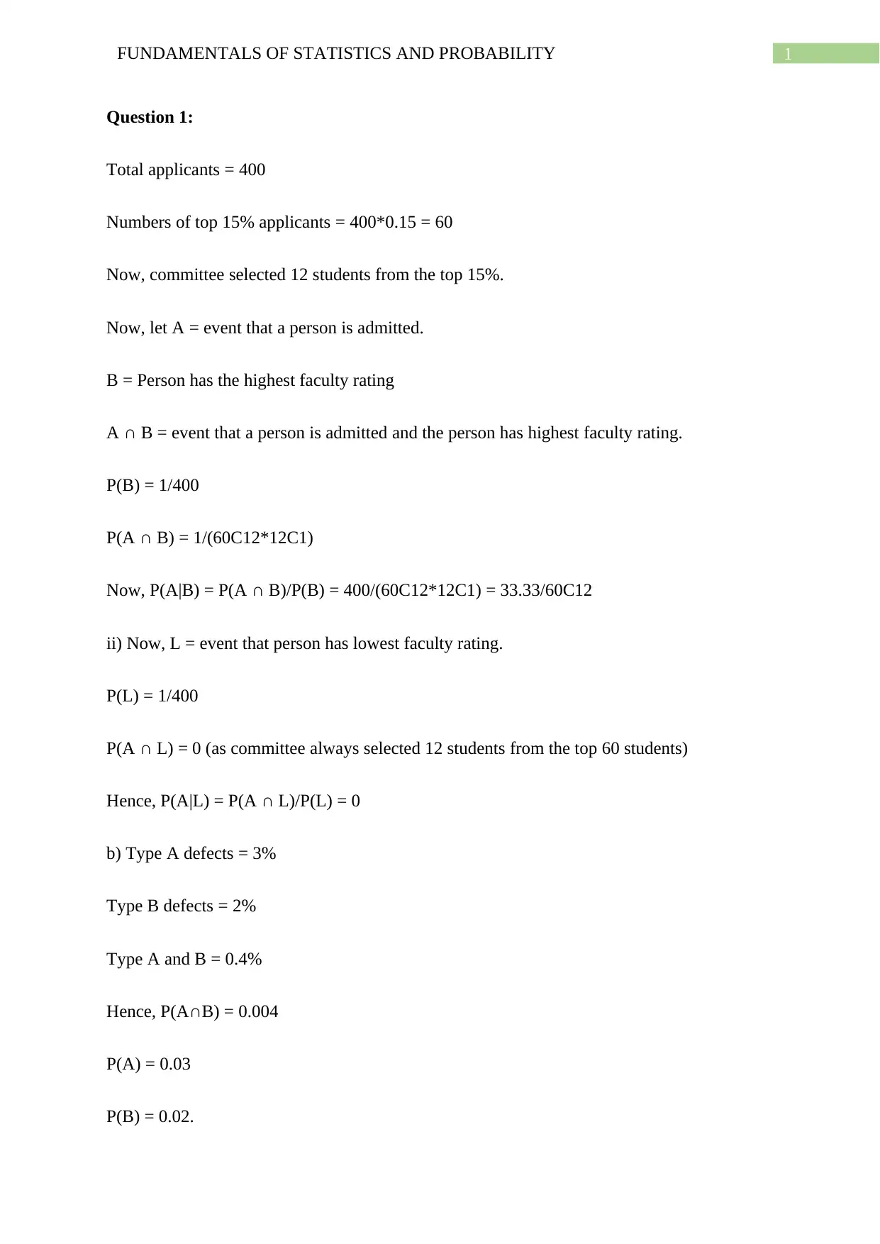
Question 1:
Total applicants = 400
Numbers of top 15% applicants = 400*0.15 = 60
Now, committee selected 12 students from the top 15%.
Now, let A = event that a person is admitted.
B = Person has the highest faculty rating
A ∩ B = event that a person is admitted and the person has highest faculty rating.
P(B) = 1/400
P(A ∩ B) = 1/(60C12*12C1)
Now, P(A|B) = P(A ∩ B)/P(B) = 400/(60C12*12C1) = 33.33/60C12
ii) Now, L = event that person has lowest faculty rating.
P(L) = 1/400
P(A ∩ L) = 0 (as committee always selected 12 students from the top 60 students)
Hence, P(A|L) = P(A ∩ L)/P(L) = 0
b) Type A defects = 3%
Type B defects = 2%
Type A and B = 0.4%
Hence, P(A∩B) = 0.004
P(A) = 0.03
P(B) = 0.02.

2FUNDAMENTALS OF STATISTICS AND PROBABILITY
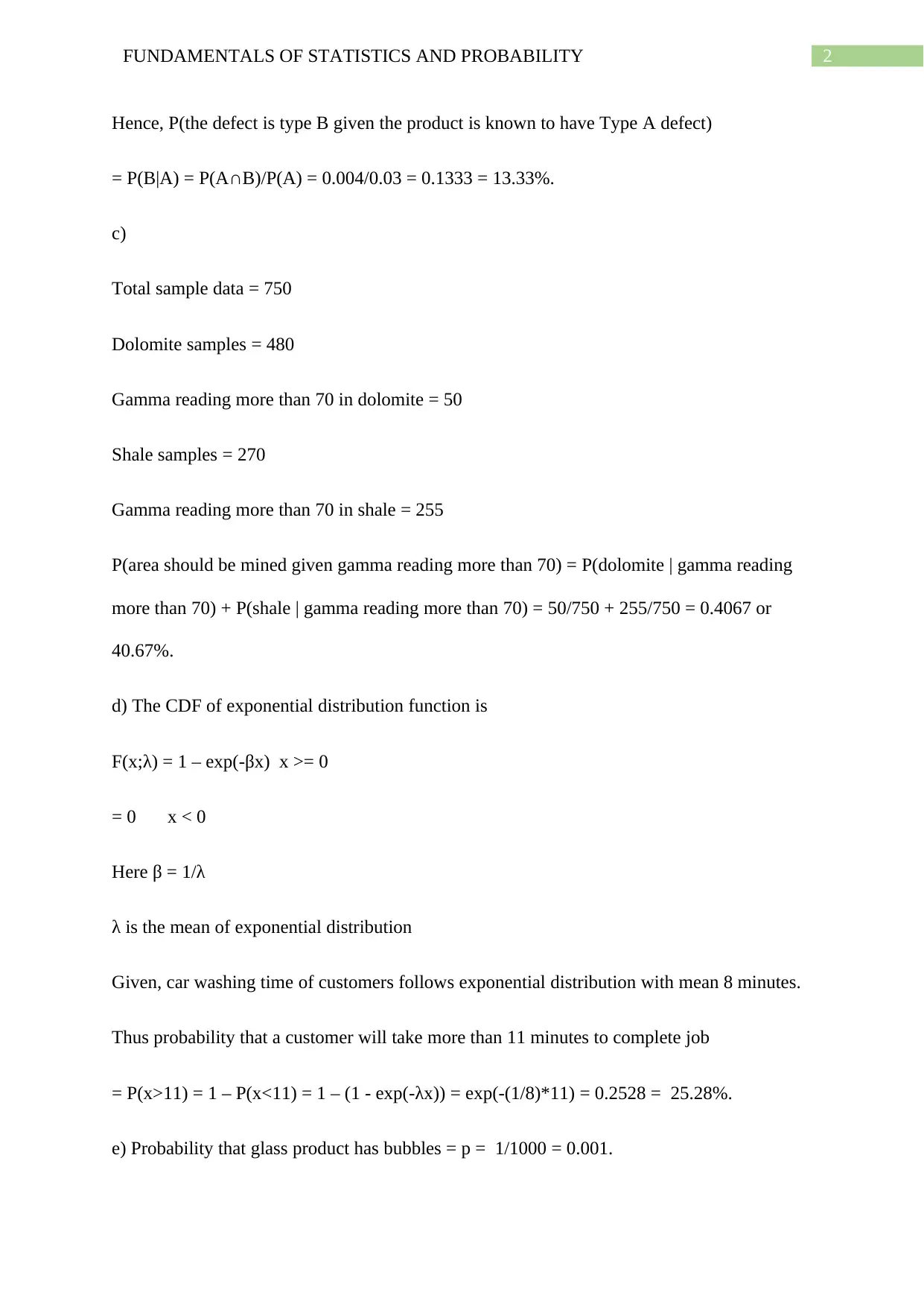
Hence, P(the defect is type B given the product is known to have Type A defect)
= P(B|A) = P(A∩B)/P(A) = 0.004/0.03 = 0.1333 = 13.33%.
c)
Total sample data = 750
Dolomite samples = 480
Gamma reading more than 70 in dolomite = 50
Shale samples = 270
Gamma reading more than 70 in shale = 255
P(area should be mined given gamma reading more than 70) = P(dolomite | gamma reading
more than 70) + P(shale | gamma reading more than 70) = 50/750 + 255/750 = 0.4067 or
40.67%.
d) The CDF of exponential distribution function is
F(x;λ) = 1 – exp(-βx) x >= 0
= 0 x < 0
Here β = 1/λ
λ is the mean of exponential distribution
Given, car washing time of customers follows exponential distribution with mean 8 minutes.
Thus probability that a customer will take more than 11 minutes to complete job
= P(x>11) = 1 – P(x<11) = 1 – (1 - exp(-λx)) = exp(-(1/8)*11) = 0.2528 = 25.28%.
e) Probability that glass product has bubbles = p = 1/1000 = 0.001.

3FUNDAMENTALS OF STATISTICS AND PROBABILITY
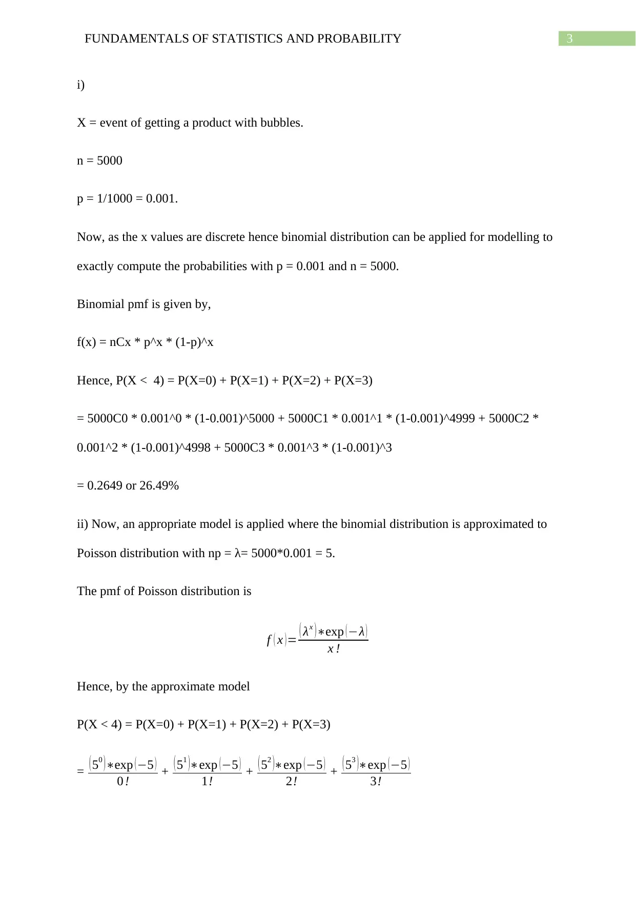
i)
X = event of getting a product with bubbles.
n = 5000
p = 1/1000 = 0.001.
Now, as the x values are discrete hence binomial distribution can be applied for modelling to
exactly compute the probabilities with p = 0.001 and n = 5000.
Binomial pmf is given by,
f(x) = nCx * p^x * (1-p)^x
Hence, P(X < 4) = P(X=0) + P(X=1) + P(X=2) + P(X=3)
= 5000C0 * 0.001^0 * (1-0.001)^5000 + 5000C1 * 0.001^1 * (1-0.001)^4999 + 5000C2 *
0.001^2 * (1-0.001)^4998 + 5000C3 * 0.001^3 * (1-0.001)^3
= 0.2649 or 26.49%
ii) Now, an appropriate model is applied where the binomial distribution is approximated to
Poisson distribution with np = λ= 5000*0.001 = 5.
The pmf of Poisson distribution is
f ( x )= ( λx )∗exp (−λ )
x !
Hence, by the approximate model
P(X < 4) = P(X=0) + P(X=1) + P(X=2) + P(X=3)
= ( 50 )∗exp (−5 )
0 ! + ( 51 )∗exp ( −5 )
1! + ( 52 )∗exp (−5 )
2! + ( 53 )∗exp (−5 )
3!

4FUNDAMENTALS OF STATISTICS AND PROBABILITY
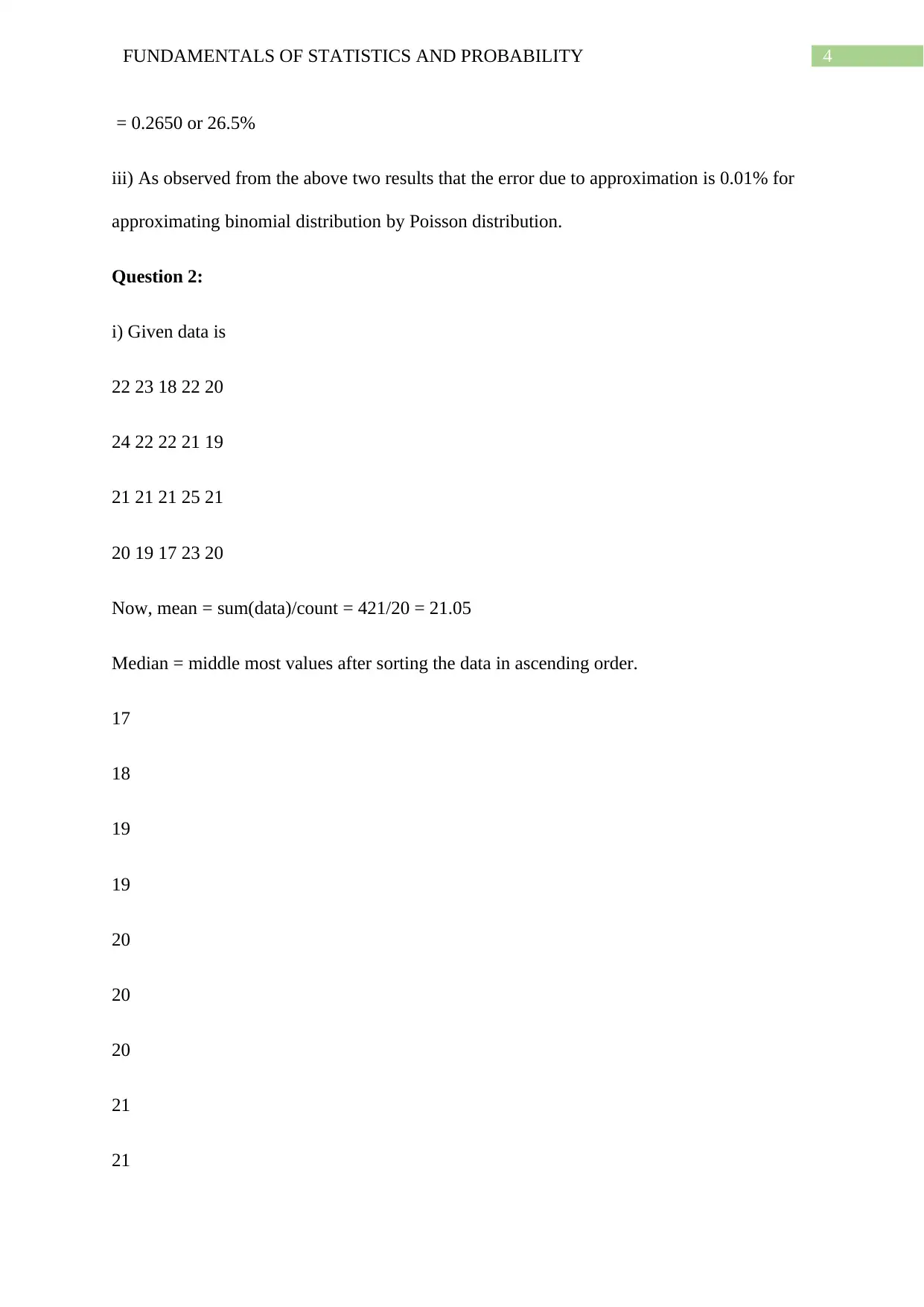
= 0.2650 or 26.5%
iii) As observed from the above two results that the error due to approximation is 0.01% for
approximating binomial distribution by Poisson distribution.
Question 2:
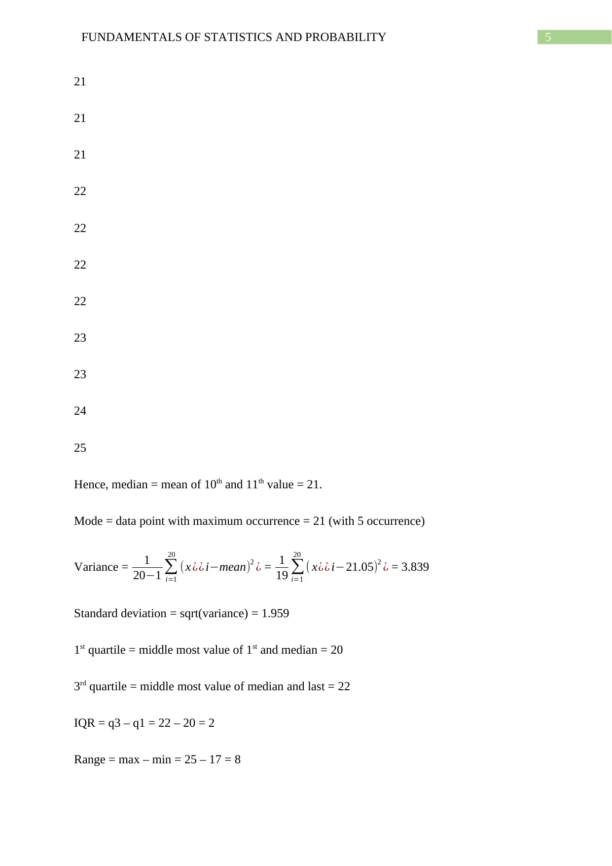
i) Given data is
22 23 18 22 20
24 22 22 21 19
21 21 21 25 21
20 19 17 23 20
Now, mean = sum(data)/count = 421/20 = 21.05
Median = middle most values after sorting the data in ascending order.
17
18
19
19
20
20
20
21
21

5FUNDAMENTALS OF STATISTICS AND PROBABILITY
21
21
21
22
22
22
22
23
23
24
25
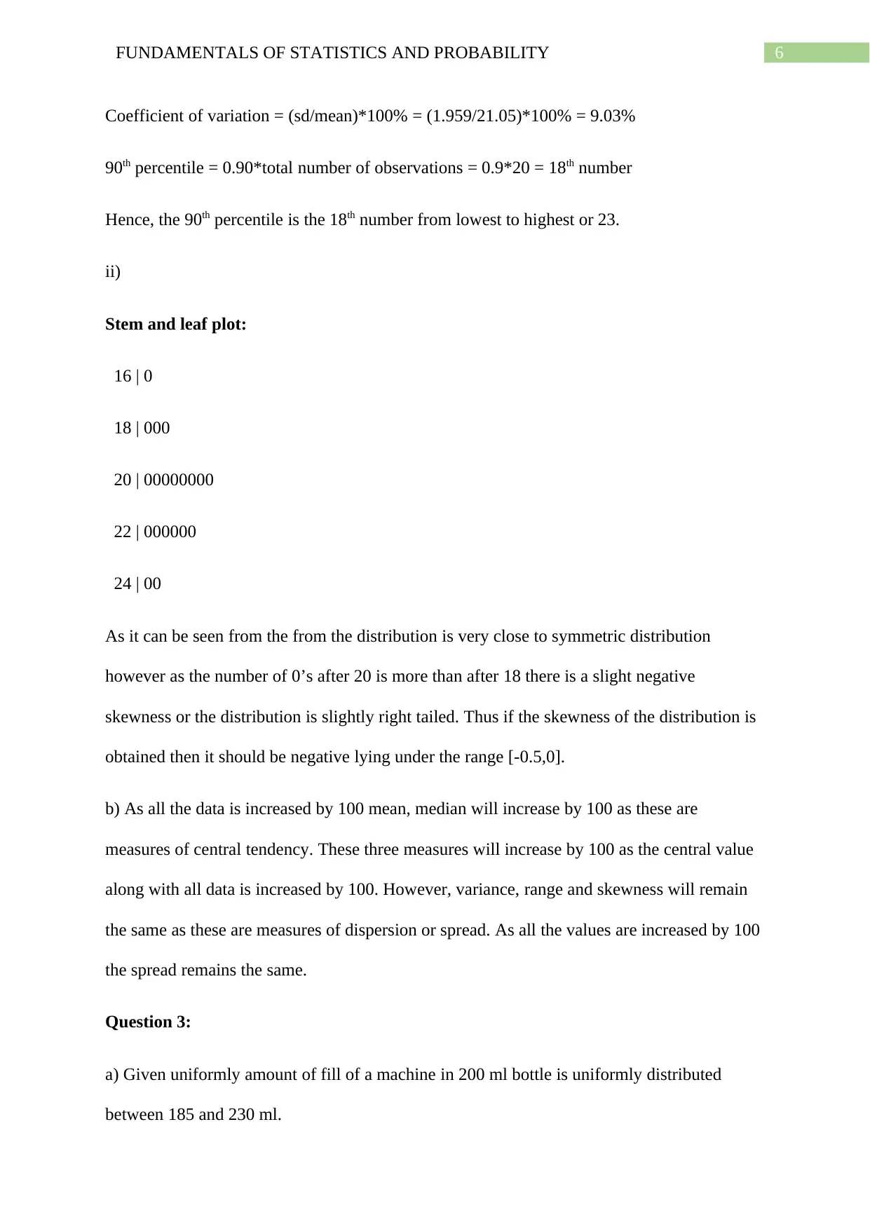
Hence, median = mean of 10th and 11th value = 21.
Mode = data point with maximum occurrence = 21 (with 5 occurrence)
Variance = 1
20−1 ∑
i=1
20
(x ¿¿ i−mean)2 ¿ = 1
19 ∑
i=1
20
( x¿¿ i−21.05)2 ¿ = 3.839
Standard deviation = sqrt(variance) = 1.959
1st quartile = middle most value of 1st and median = 20
3rd quartile = middle most value of median and last = 22
IQR = q3 – q1 = 22 – 20 = 2
Range = max – min = 25 – 17 = 8

6FUNDAMENTALS OF STATISTICS AND PROBABILITY
Coefficient of variation = (sd/mean)*100% = (1.959/21.05)*100% = 9.03%
90th percentile = 0.90*total number of observations = 0.9*20 = 18th number
Hence, the 90th percentile is the 18th number from lowest to highest or 23.
ii)
Stem and leaf plot:
16 | 0
18 | 000
20 | 00000000
22 | 000000
24 | 00
As it can be seen from the from the distribution is very close to symmetric distribution
however as the number of 0’s after 20 is more than after 18 there is a slight negative
skewness or the distribution is slightly right tailed. Thus if the skewness of the distribution is
obtained then it should be negative lying under the range [-0.5,0].
b) As all the data is increased by 100 mean, median will increase by 100 as these are
measures of central tendency. These three measures will increase by 100 as the central value
along with all data is increased by 100. However, variance, range and skewness will remain
the same as these are measures of dispersion or spread. As all the values are increased by 100
the spread remains the same.
Question 3:
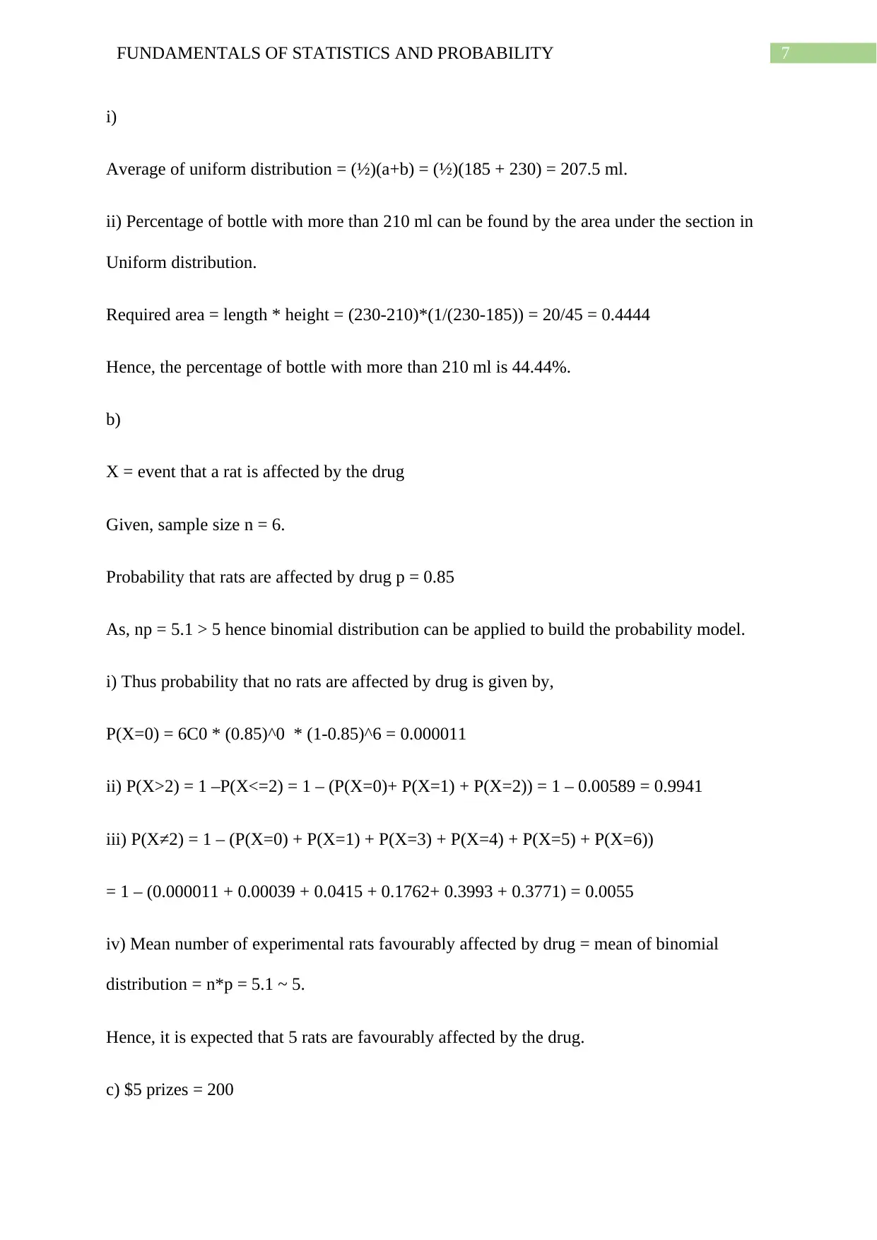
a) Given uniformly amount of fill of a machine in 200 ml bottle is uniformly distributed
between 185 and 230 ml.

7FUNDAMENTALS OF STATISTICS AND PROBABILITY
i)
Average of uniform distribution = (½)(a+b) = (½)(185 + 230) = 207.5 ml.
ii) Percentage of bottle with more than 210 ml can be found by the area under the section in
Uniform distribution.
Required area = length * height = (230-210)*(1/(230-185)) = 20/45 = 0.4444
Hence, the percentage of bottle with more than 210 ml is 44.44%.
b)
X = event that a rat is affected by the drug
Given, sample size n = 6.
Probability that rats are affected by drug p = 0.85
As, np = 5.1 > 5 hence binomial distribution can be applied to build the probability model.
i) Thus probability that no rats are affected by drug is given by,
P(X=0) = 6C0 * (0.85)^0 * (1-0.85)^6 = 0.000011
ii) P(X>2) = 1 –P(X<=2) = 1 – (P(X=0)+ P(X=1) + P(X=2)) = 1 – 0.00589 = 0.9941
iii) P(X≠2) = 1 – (P(X=0) + P(X=1) + P(X=3) + P(X=4) + P(X=5) + P(X=6))
= 1 – (0.000011 + 0.00039 + 0.0415 + 0.1762+ 0.3993 + 0.3771) = 0.0055
iv) Mean number of experimental rats favourably affected by drug = mean of binomial
distribution = n*p = 5.1 ~ 5.
Hence, it is expected that 5 rats are favourably affected by the drug.
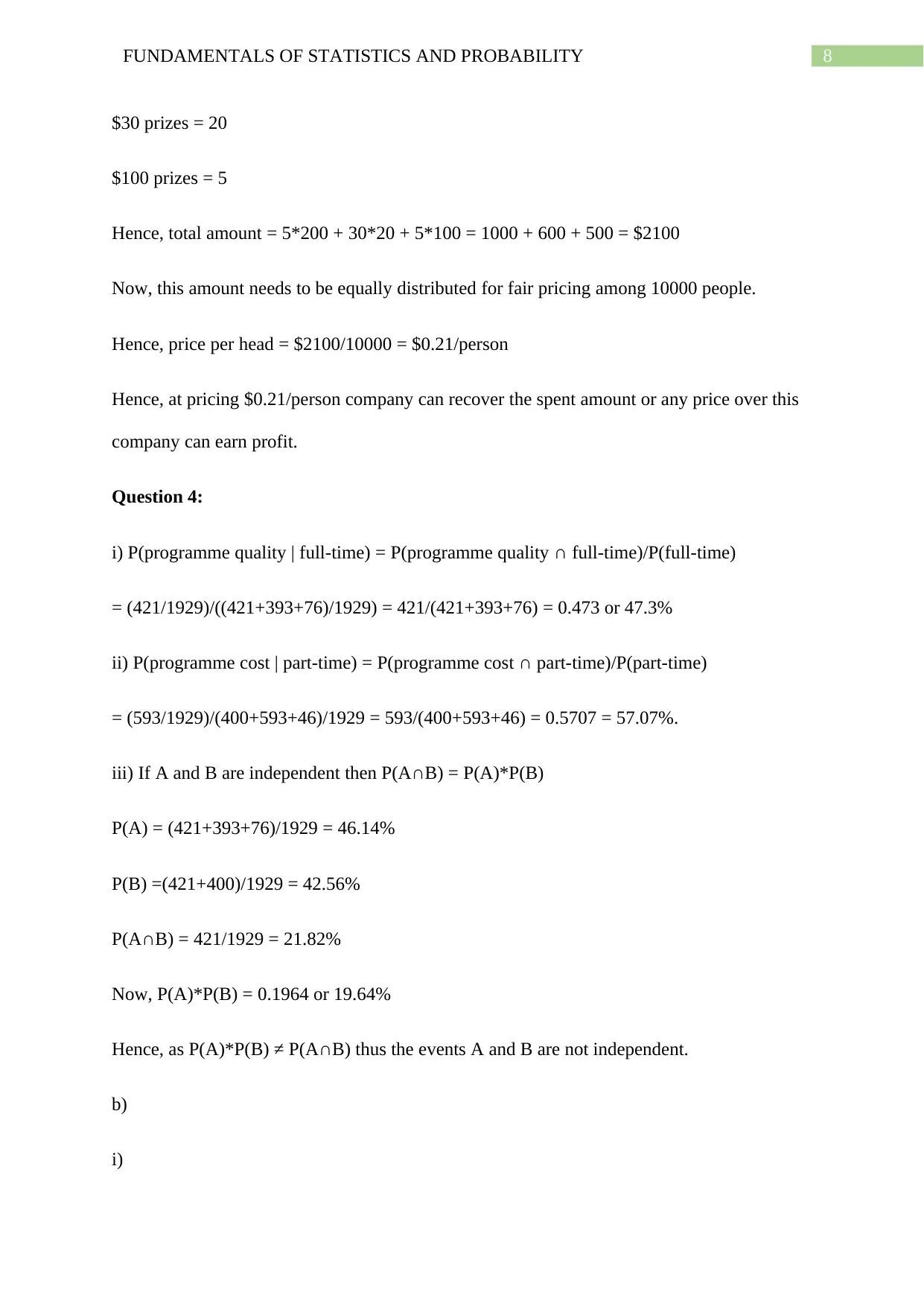
c) $5 prizes = 200

8FUNDAMENTALS OF STATISTICS AND PROBABILITY
$30 prizes = 20
$100 prizes = 5
Hence, total amount = 5*200 + 30*20 + 5*100 = 1000 + 600 + 500 = $2100
Now, this amount needs to be equally distributed for fair pricing among 10000 people.
Hence, price per head = $2100/10000 = $0.21/person
Hence, at pricing $0.21/person company can recover the spent amount or any price over this
company can earn profit.
Question 4:
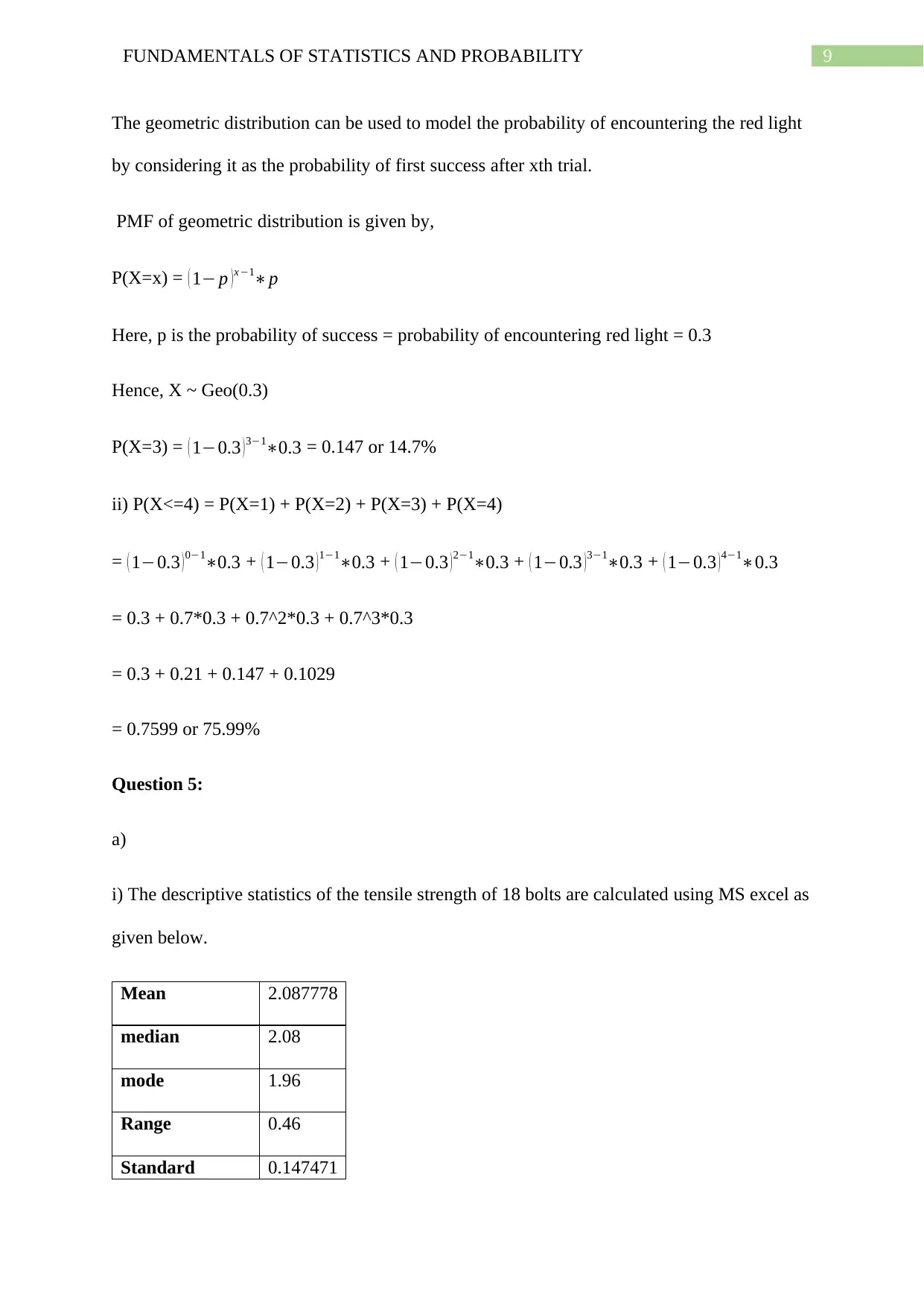
i) P(programme quality | full-time) = P(programme quality ∩ full-time)/P(full-time)
= (421/1929)/((421+393+76)/1929) = 421/(421+393+76) = 0.473 or 47.3%
ii) P(programme cost | part-time) = P(programme cost ∩ part-time)/P(part-time)
= (593/1929)/(400+593+46)/1929 = 593/(400+593+46) = 0.5707 = 57.07%.
iii) If A and B are independent then P(A∩B) = P(A)*P(B)
P(A) = (421+393+76)/1929 = 46.14%
P(B) =(421+400)/1929 = 42.56%
P(A∩B) = 421/1929 = 21.82%
Now, P(A)*P(B) = 0.1964 or 19.64%
Hence, as P(A)*P(B) ≠ P(A∩B) thus the events A and B are not independent.
b)
i)

9FUNDAMENTALS OF STATISTICS AND PROBABILITY
The geometric distribution can be used to model the probability of encountering the red light
by considering it as the probability of first success after xth trial.
PMF of geometric distribution is given by,
P(X=x) = ( 1− p ) x−1∗p
Here, p is the probability of success = probability of encountering red light = 0.3
Hence, X ~ Geo(0.3)
P(X=3) = ( 1−0.3 )3−1∗0.3 = 0.147 or 14.7%
ii) P(X<=4) = P(X=1) + P(X=2) + P(X=3) + P(X=4)
= ( 1−0.3 ) 0−1∗0.3 + ( 1−0.3 ) 1−1∗0.3 + ( 1−0.3 ) 2−1∗0.3 + ( 1−0.3 ) 3−1∗0.3 + ( 1−0.3 ) 4−1∗0.3
= 0.3 + 0.7*0.3 + 0.7^2*0.3 + 0.7^3*0.3
= 0.3 + 0.21 + 0.147 + 0.1029
= 0.7599 or 75.99%
Question 5:
a)
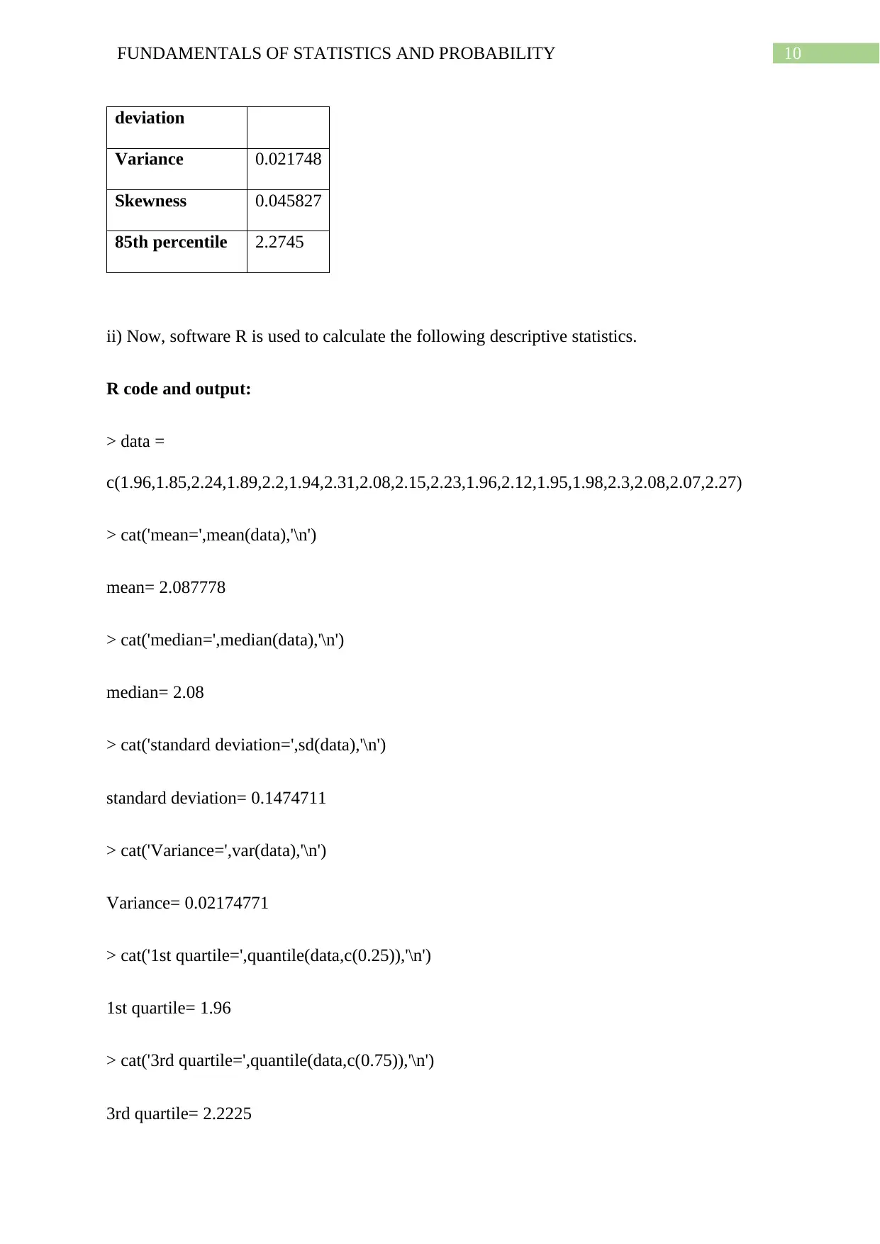
i) The descriptive statistics of the tensile strength of 18 bolts are calculated using MS excel as
given below.
Mean 2.087778
median 2.08
mode 1.96
Range 0.46
Standard 0.147471

10FUNDAMENTALS OF STATISTICS AND PROBABILITY
deviation
Variance 0.021748
Skewness 0.045827
85th percentile 2.2745
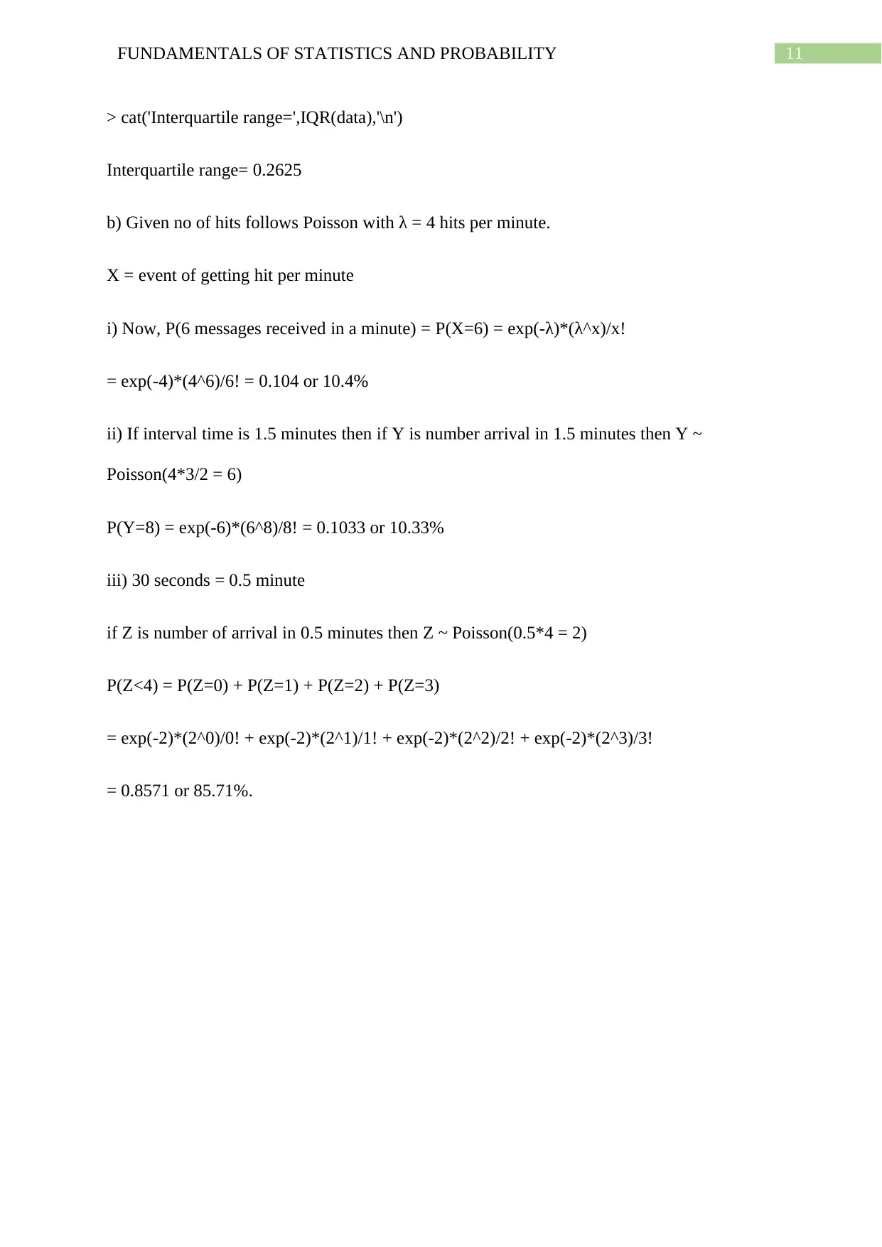
ii) Now, software R is used to calculate the following descriptive statistics.
R code and output:
> data =
c(1.96,1.85,2.24,1.89,2.2,1.94,2.31,2.08,2.15,2.23,1.96,2.12,1.95,1.98,2.3,2.08,2.07,2.27)
> cat('mean=',mean(data),'\n')
mean= 2.087778
> cat('median=',median(data),'\n')
median= 2.08
> cat('standard deviation=',sd(data),'\n')
standard deviation= 0.1474711
> cat('Variance=',var(data),'\n')
Variance= 0.02174771
> cat('1st quartile=',quantile(data,c(0.25)),'\n')
1st quartile= 1.96
> cat('3rd quartile=',quantile(data,c(0.75)),'\n')
3rd quartile= 2.2225

11FUNDAMENTALS OF STATISTICS AND PROBABILITY
> cat('Interquartile range=',IQR(data),'\n')
Interquartile range= 0.2625
b) Given no of hits follows Poisson with λ = 4 hits per minute.
X = event of getting hit per minute
i) Now, P(6 messages received in a minute) = P(X=6) = exp(-λ)*(λ^x)/x!
= exp(-4)*(4^6)/6! = 0.104 or 10.4%
ii) If interval time is 1.5 minutes then if Y is number arrival in 1.5 minutes then Y ~
Poisson(4*3/2 = 6)
P(Y=8) = exp(-6)*(6^8)/8! = 0.1033 or 10.33%
iii) 30 seconds = 0.5 minute
if Z is number of arrival in 0.5 minutes then Z ~ Poisson(0.5*4 = 2)
P(Z<4) = P(Z=0) + P(Z=1) + P(Z=2) + P(Z=3)
= exp(-2)*(2^0)/0! + exp(-2)*(2^1)/1! + exp(-2)*(2^2)/2! + exp(-2)*(2^3)/3!
= 0.8571 or 85.71%.