2018 Further Engineering Mathematics Assignment Solution

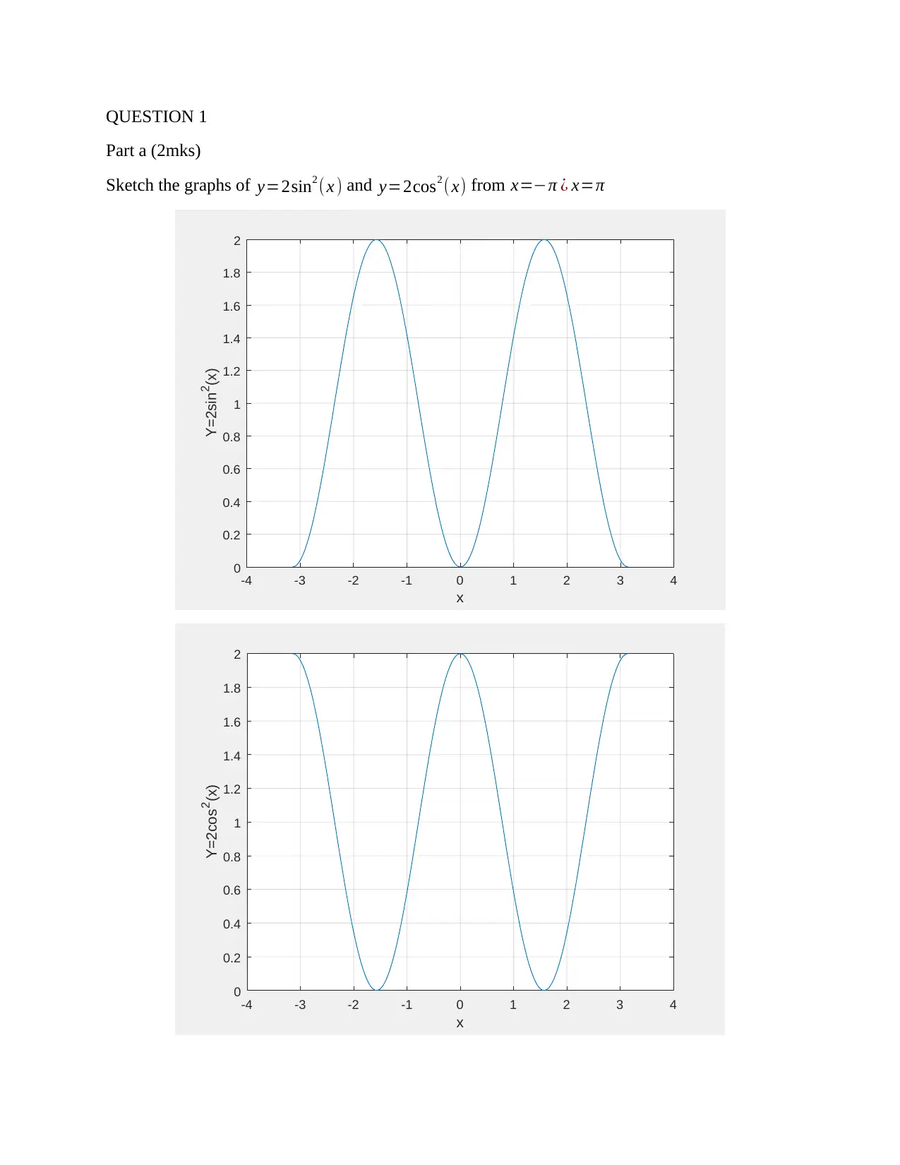
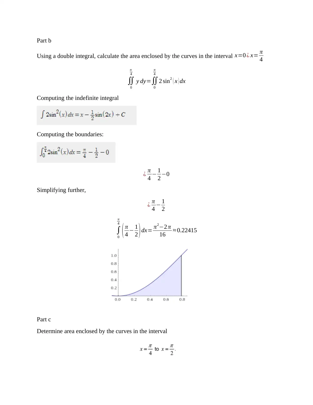
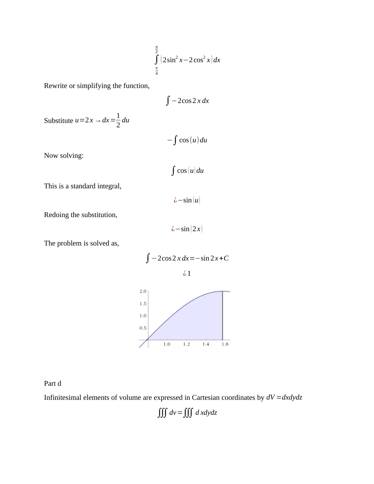
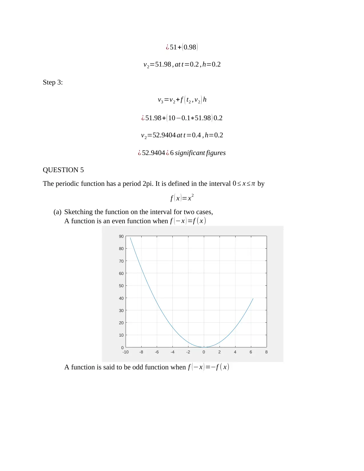
This document presents a comprehensive solution to a Further Engineering Mathematics assignment. The solution includes detailed calculations and explanations for various mathematical concepts. Part (a) provides sketched graphs of trigonometric functions. Part (b) and (c) demonstrate the calculation of areas using double integrals. Part (d) involves the calculation of volume using a triple integral. Part (e) is not fully addressed in the provided text. Question 2 explores line integrals, curve lengths, and work done by a force. Question 3 utilizes the power method to find the dominant eigenvalue and eigenvector of a matrix. Question 4 applies the 2nd Runge-Kutta method to solve an initial value problem. Finally, Question 5 analyzes a periodic function using Fourier series, including sketching and coefficient calculations.

2018
INSTITUTIONAL AFFILIATION
FACULTY OR DEPARTMENT
COURSE ID & NAME
TITLE:
FUTURE ENGINEERING MATHEMATICS
STUDENT NAME
STUDENT ID NUMBER
PROFESSOR (TUTOR)
DATE OF SUBMISSION

QUESTION 1
Part a (2mks)
Sketch the graphs of y=2sin2 ( x ) and y=2cos2 (x) from x=−π ¿ x=π
-4 -3 -2 -1 0 1 2 3 4
x
0
0.2
0.4
0.6
0.8
1
1.2
1.4
1.6
1.8
2
Y=2sin 2 (x)
-4 -3 -2 -1 0 1 2 3 4
x
0
0.2
0.4
0.6
0.8
1
1.2
1.4
1.6
1.8
2
Y=2cos2(x)

Part b
Using a double integral, calculate the area enclosed by the curves in the interval x=0 ¿ x= π
4
∬
0
π
4
y dy=∬
0
π
4
2 sin2 ( x ) dx
Computing the indefinite integral
Computing the boundaries:
¿ π
4 − 1
2 −0
Simplifying further,
¿ π
4 − 1
2
∫
0
π
4
( π
4 − 1
2 )dx= π2−2 π
16 ≈ 0.22415
Part c
Determine area enclosed by the curves in the interval

∫
π
4
π
2
( 2sin2 x−2 cos2 x ) dx
Rewrite or simplifying the function,
∫−2cos 2 x dx
Substitute u=2 x →dx =1
2 du
−∫cos (u) du
Now solving:
∫cos ( u ) du
This is a standard integral,
¿−sin ( u )
Redoing the substitution,
¿−sin ( 2 x )
The problem is solved as,
∫−2cos 2 x dx=−sin 2 x +C
¿ 1
Part d
Infinitesimal elements of volume are expressed in Cartesian coordinates by dV =dxdydz
∭dv =∭ d xdydz

¿∫
0
3 x
∫
2.5
2.5
∫
ex
❑
dv
Part e
Infinitesimal elements of volume are expressed in spherical polar coordinates as
dV =r2 sin (θ) drd θ d φ
QUESTION 2
Part a
Evaluate I=∫
c
❑
( 2 xy + y ) dxalong the path C described parametrically by x=t2 , y= 1
t2 ¿ t=C ¿ 4
Solution

¿∨⃗ r ( t ) ∨¿= √ ( dx
dt )2
+ ( dy
dt )2
I =∫
c
❑
( 2t2 . 1
t2 + 1
t2 )||⃗r ( t )||dt
dx
dt =2t , dy
dt =−2
t3
||⃗r ( t )||= √ ( 2t ) 2+ ( −2
t3 )
2
= √ 4 t2+ 4
t6
||⃗r ( t )||=2 ( √ 1+t8
t6 )
I =∫
c
4
( 2+ 1
t2 )∗2 ( √ 1+t8
t6 ) dt
The line integral is given as,
I =∫
c
4
2 ( 2+ 1
t2 ) ( √ 1+t8
t6 ) dt
Part b
Calculate the length of the curve, y=ln |sec ( x )|from x=0 ¿ x= π
3
y=ln |sec ( x )|0 ≤ x ≤ π
3
For the given interval,
|sec ( x )|=sec ( x )
y' = 1
sec ( x ) ( sec x )'=sec x ( tan x
sec x )=tan x
length=∫ √ ( 1+ ( y' ) 2
) dx
y=ln |sec x|∧x=0¿ x= π
3
¿∫ √1+tan2 x dx for thelimits

¿∫ sec x dx for thelimita
¿ [ ln ( sec x + tan x ) ] , between x=0 ¿ x= π
3
¿ ln ( sec ( π
3 ) + tan ( π
3 ))
sec ( π
3 )= √ 1+ tan2 π
3 = √ 1+3=2
¿ ln ( 2+1 )=ln ( 3 )=1.09
Part c
Find the work done by the force F= ( 3 xy +4 ) i+ y3 j moving anticlockwise around the boundaries
of the triangle defined by the points (0,0), (4,0), and (4,4).
SOLUTION
Denoting the points as C1, C2, and C3.
C1= ( 0,0 ) C2 = ( 4,4 ) C3= ( 4,0 )
Dealing with the line segments
C= ( 0,0 ) ¿ ( 4,4 )∧ ( 4,4 ) ¿ ( 4,0 )∧ ( 4,0 ) ¿ ( 0,0 )
∫
∁
❑
fds=∫
C1
❑
fds+∫
C2
❑
fds+∫
C3
❑
fds
F= ( 3 xy +4 ) i+ y3 j
∇ f = ( 3 xy+ 4 , y3 ) =F
f x=3 y
f y=3 x ,3 y2
c1= {x=0. ( 1−t ) +2 t
y=0. ( 1−t ) +t }
c2= {x=4 . ( 1−t )+ 2t
y =4 . ( 1−t ) +t }
c3= {x=4 . ( 1−t )+ 2t
y=0. ( 1−t ) +t }

∫
∁
❑
fds=∫
0,0
4,4
❑+∫
4,4
4,0
fds+∫
4,0
0,0
fds
The gradient vector field is,
¿ 3 √ 5∫ ( 4 t2−t2 ) √ 5 dt +∫ ( 2−t2 ) − ( t +1 ) 2 √ 2 dt+∫ ( 1−t ) 2−4 ¿ ¿
¿ 3 √ 5∫
0
1
t2 dt + √ 2∫
0
1
( 3−6 t ) dt+ √ 5∫
0
1
(−3+6 t=3 t2 ) dt
¿ 6
Part d
By using Green’s Theorem, verify this result with a double integral over the area of the triangle.
¿∫
0
4
( 14+10 t ) dt=6
QUESTION 3
Use the power method to find, correct to 3 decimal places, the dominant eigenvalue, and a
corresponding eigenvector of the matrix.
[ 0 11 −5
−2 17 −7
−4 −26 −10 ]T
Start with the initial vector [1,1,1]T and work to 3 decimal places throughout.

AT = [ 0 11 −5
−2 17 −7
−4 −26 −10 ]T
A=
[ 0 −2 −4
11 17 −26
−5 −7 −10 ]T
initial approximations , x0= [ 1
1
1 ] ,
Taking out the largest element of the resultant matrix,
x1= A ~x1=
( 0 −2 −4
11 17 −26
−5 −7 −10 )(1
1
1 )= ( −6
2
−22 )=−22 ( 0.2727
−0.0909
1.0000 )
Using the resulting matrix as the new initial vector for the next iteration,
x2= A ~x2=
( 0 −2 −4
11 17 −26
−5 −7 −10 )( 0.2727
−0.0909
1.0000 )=
( −3.8182
−24.5456
−10.7272 )=−24.5456 (0.1556
1.000
0.4370 )
Repeating the same procedure to obtain an iteration of the sequence,
x3= A ~x3=
( 0 −2 −4
11 17 −26
−5 −7 −10 )(0.1556
1.000
0.4370 )=
( −3.7481
7.3483
−12.1481 )=−12.1481 ( 0.3085
−0.6049
1.000 )
x3= A ~x3=
( 0 −2 −4
11 17 −26
−5 −7 −10 )( 0.3085
−0.6049
1.0000 )=
( −2.7902
−32.8893
−7.3084 )=−32.8893 (0.0848
1.000
0.2222 )
x4 =A ~x4 =
( 0 −2 −4
11 17 −26
−5 −7 −10 )(0.0848
1.000
0.2222 )=
(−2.8888
12.1556
−9.6463 )=12.1556 (−0.2377
1.000
−0.7936 )
x4 =A ~x4 =
( 0 −2 −4
11 17 −26
−5 −7 −10 )(−0.2377
1.000
−0.7936 )=
( 1.1743
35.0186
2.1239 )=35.0186 (0.0335
1.000
0.0607 )
x5= A ~x5=
( 0 −2 −4
11 17 −26
−5 −7 −10 )(0.0335
1.000
0.0607 )=
(−2.2426
15.7919
−7.7742 )=15.7919 (−0.1420
1.000
−0.4923 )

x6= A ~x6= ( 0 −2 −4
11 17 −26
−5 −7 −10)(−0.1420
1.000
−0.4923 )= (−0.0308
28.2374
−1.3671 )=28.2374 (−0.0011
1.0000
−0.0484 )
x7= A ~x7= ( 0 −2 −4
11 17 −26
−5 −7 −10 )( −0.0011
1.0000
−0.0484 )= (
−1.8063
18.2468
−6.5104 ) =18.2468 (
−0.0990
1.0000
−0.3568 )
x8= A ~x8= ( 0 −2 −4
11 17 −26
−5 −7 −10)(−0.0990
1.0000
−0.3568 )= (−0.5728
25.1878
−2.9370 )=25.1878 (−0.0227
1.0000
−0.1166 )
x9= A ~x9= ( 0 −2 −4
11 17 −26
−5 −7 −10)(
−0.0227
1.0000
−0.1166 )= (
−1.5336
19.7816
−5.7203 )=19.7816 (
−0.0775
1.0000
−0.2892 )
x10= A ~x10=
( 0 −2 −4
11 17 −26
−5 −7 −10 )(−0.0775
1.0000
−0.2892 )= (−0.8433
23.6656
−3.7207 )=23.6656 (−0.0356
1.0000
−0.1572 )
To obtain the eigen values and dominant eigen vector, the iterations are carried out
progressively. The dominant eigenvector is obtained as,
23.6656 … . dominant eigen value
(−0.0356
1.0000
−0.1572 )=dominant eigenvector
QUESTION 4
Consider the initial value problem,
dv
dt =10−0.1 v with vo =50 at to=0
Using the 2nd Runge-Kutta method to calculate the approximate value of v at t=0.4, using step
size h=0.2 and working to six significant figures.
The modified Euler’s method is the second-order Runge Kutta method,

X n+1=X n+ ∆ t
2 [ f ( xn ,tn ) + f ( xn+∆ tf ( xn ,tn ) , tn + ∆t ) ]
xi+1
¿ =xi−∆ t xi
2
To solve the ode using 2nd order RK method,
Initialization,
k =0 , h= b−t0
n y ( tk ) = yk
Predict the solution,
yk +1= yk + hf ( tk +1 , yk +1 , p )
2
Increment the value,
tk+1=tk +h , k =k +1
Using the algorithm to find the solution,
dv
dt =10−0.1 v , , v0 =50 at t0=0 h=0.2
Step 1:
V i+ 1=vi + f ( ti , vi ) h
vi =50+f ( 0,50 ) 0.2
¿ 50+ ( 10−0.1∗50 ) 0.2
¿ 50+ ( 5 ) 0.2
vi =51
Step 2:
v2=v1 +f ( t1 , v1 ) h
¿ 51+ ( 10−0.1∗51 ) 0.2

¿ 51+ ( 0.98 )
v2=51.98 , at t=0.2 , h=0.2
Step 3:
v3 =v2 +f ( t2 , v2 ) h
¿ 51.98+ ( 10−0.1∗51.98 ) 0.2
v2=52.9404 at t=0.4 , h=0.2
¿ 52.9404 ¿ 6 significant figures
QUESTION 5
The periodic function has a period 2pi. It is defined in the interval 0 ≤ x ≤ π by
f ( x )=x2
(a) Sketching the function on the interval for two cases,
A function is an even function when f ( −x ) =f (x )
-10 -8 -6 -4 -2 0 2 4 6 8
0
10
20
30
40
50
60
70
80
90
A function is said to be odd function when f ( −x ) =−f ( x)

-10 -8 -6 -4 -2 0 2 4 6 8
-90
-80
-70
-60
-50
-40
-30
-20
-10
0
(b) Fourier coefficients of the two functions.
The Fourier cosine series describes an even function and the Fourier sine series describes
an odd function. For an odd function
f ( x ) = a0
2 +∑
n=1
∞
an cos ( nπ
L ) x
For an even function,
f ( x ) =∑
n=1
∞
bn sin ( nπ
L ) x
Using the Fourier series, the function in part a is an even function.
a0= 2
1∫
0
π
x2 dx= 2
3 π3
an=2∫
0
π
x2 cos ( nπx ) dx
Using integration by parts
an= x2 sin nπx
πn −∫ 2 x sin nπx
πn dx
Now solving,
∫ 2 x sin nπx
πn dx
Applying linearity,
¿ 2
nπ ∫ x sin nπx dx
bn= 2
π ∫
0
π
x sin nx dx

¿ 2
π ( [ −xcos nx
n ]0
π
−∫
0
π
−cos nx
n dx )
¿ 2
π ∗
( 1
n [ −π cos nπ ] + [ sin nx
n2 ] 0
π
)
¿− 2
n cos nπ
¿
{−2
n if n is even
2
n if n is odd
(c) Given that
Is a periodic function of period 2pi, by using integration by parts when required, calculate
the Fourier coefficients for the function, g(x), and express it as Fourier series expansion.
g ( x ) =∫
0
π
∫
π
2 π
( x ) ( −x ) dx
The Fourier series is given as
g ( x )=b1 sin x+ b2 sin2 x +b3 sin 3 x +…
g ( x )=2 sin x −sin 2 x + 2
3 sin 3 x−1
2 sin 4 x + 2
5 sin 5 x+…
(d) Deduce that π 2
8 = {1+ 1
9 + 1
25 + 1
49 + … }=∑
n=1
∞ 1
( 2 n−1 ) 2
Let function f(x) be an even function,
f ( x )= a0
2 +∑
n=1
∞
sin nx
a0= 1
π ∫
−π
π
x2 dx = 2
π ∫
0
π
x2 dx
¿ 2
π [ x3
3 ]0
π
=
2
π ∗π3
3 = 2 π2
3
an= 1
π ∫
−π
π
x2 cos nx dx= 2
π ∫
0
π
x2 cos nx dx
Using integration by parts,

¿ 2
π [ x2
n sin nx −2
n ∫ x sin nx dx ]0
π
¿ 2
π [ x2
n sin nx −2
n ( −x
n cos nx −∫ −1
n cos nx dx ) ]0
π
¿ 2
n [ x2
n sin nx+ 2 x
n cos nx− 2
n3 sin nx ]0
π
¿ 4
n2 cos nπ = 4
n2 (−1 )n
Substitution the values of f(x), a0 and an,
x2= π 2
3 +4 ∑
n=1
∞ (−1 )n
n2 cos nx
Substituting x= π
2
Substituting x=π,
Adding the above equations
π2
6 ∧π2
12
,
Therefore,

(e) Write down the values of ¿ ao ,a1 , … . , a5 and ¿ b1 , b2 , … . ,b5 correct to four significant
figures.

MATLAB implementation
x1= -pi:pi/10:pi;
gx1=(4/pi)*((sin(x1)/1)+(sin(3*x1)/3)+(sin(5*x1)/5)+(sin(7*x1)/7));
plot(x1,gx1)
grid on
-4 -3 -2 -1 0 1 2 3 4
-1.5
-1
-0.5
0
0.5
1
1.5