SPSS Project: Forecasting Gazprom's Sales Trends and Analysis

This project analyzes the sales trends of Gazprom, a major natural gas producer, using time series analysis and SPSS. The assignment explores various forecasting techniques, including ARIMA models, weighted moving averages, and simple exponential smoothing, to predict future sales. The report details the data used, justification for the chosen methodologies, and a cost-benefit assessment of each approach. Findings from each forecasting method are presented, including model statistics and interpretations of the results. The project concludes with a summary of the sales trends and provides recommendations for future sales predictions. The analysis includes detailed tables and charts generated from SPSS, offering a comprehensive understanding of the sales patterns and forecasting outcomes.

SPSS CONSTRUCTION OF THE
COMPANY'S SALES TREND

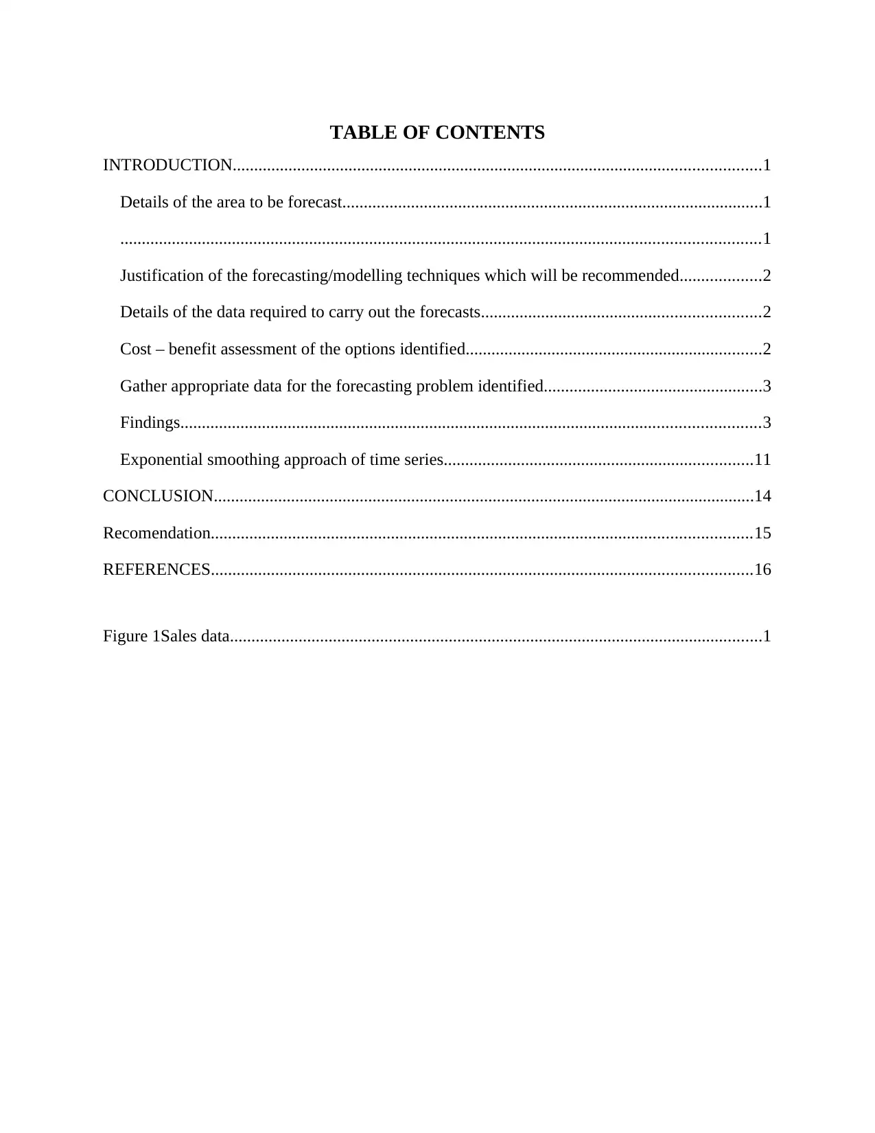
TABLE OF CONTENTS
INTRODUCTION...........................................................................................................................1
Details of the area to be forecast..................................................................................................1
.....................................................................................................................................................1
Justification of the forecasting/modelling techniques which will be recommended...................2
Details of the data required to carry out the forecasts.................................................................2
Cost – benefit assessment of the options identified.....................................................................2
Gather appropriate data for the forecasting problem identified...................................................3
Findings.......................................................................................................................................3
Exponential smoothing approach of time series........................................................................11
CONCLUSION..............................................................................................................................14
Recomendation..............................................................................................................................15
REFERENCES..............................................................................................................................16
Figure 1Sales data............................................................................................................................1

INTRODUCTION
Trend analysis is the one of the most important approach that is used for making
prediction in the business. In the current report Gazpom company is taken which is well known
around the world for natural gas production and transportation. In the current report, different
approaches of time series are used for making predictions. It is observed that all approaches are
giving same results. Techniques applied for time series are ARIMA model, weighted moving
average and simple exponential smoothing method. There are some merits and demrits of these
approahces and same are taken in to consideration while doing time series analysis. At end of the
report, conclusion is formed and recommendation is made.
Details of the area to be forecast
Gazprom is one of Russian largest natural gas producer. It is involved in extraction,
production and transportation of natural gas (Open joint stock company gazprom 1999
consolidated financial reports, 1999). Demand of natural gas is highly affected by flcutuation in
its price and global economic conditions. Sales is prone to high level of uncertainity and due to
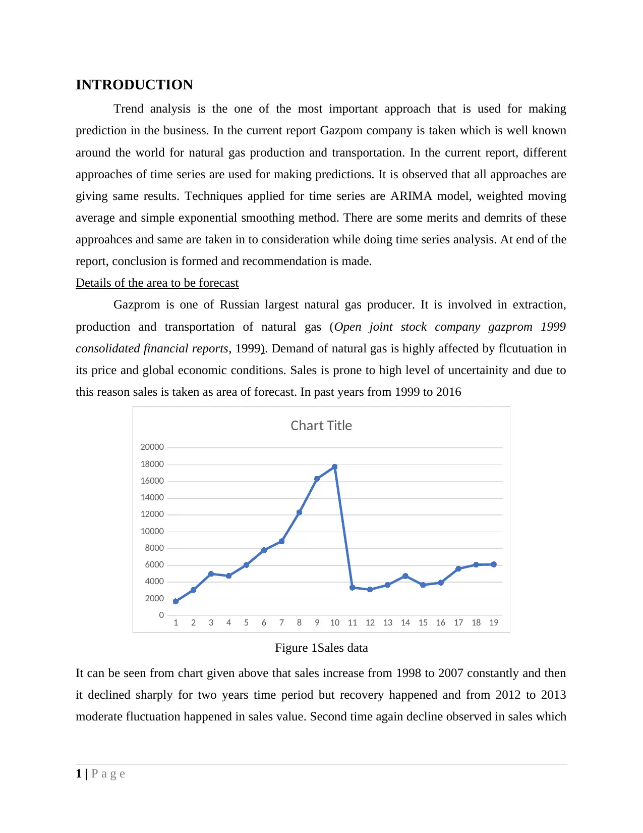
this reason sales is taken as area of forecast. In past years from 1999 to 2016
1 2 3 4 5 6 7 8 9 10 11 12 13 14 15 16 17 18 19
0
2000
4000
6000
8000
10000
12000
14000
16000
18000
20000
Chart Title
Figure 1Sales data
It can be seen from chart given above that sales increase from 1998 to 2007 constantly and then
it declined sharply for two years time period but recovery happened and from 2012 to 2013
moderate fluctuation happened in sales value. Second time again decline observed in sales which
1 | P a g e

was very moderate as sales tumbeled by moderate percentage and still there is very low growth
in sales. Hence, due to this reason sales value of the firm is considered for making prediction.
Justification of the forecasting/modelling techniques which will be recommended
There are three forecast modeling approaches that are recommended for making
prediction. ARIMA model: ARIMA model is recommended because it is an apprach under which
auto regression and moving average approaches are used for making predictions. It must
be noted that under this approach seasonal decomposition is also done and under this
different factors due to which fluctuation happened in data set are identified and removed
like seasonal and cyclical factors etc (Aoki, 2013). Hence, there is high reliability of
mentioned approach for making prediction. Weighted moving average approach: It is another apporach that is used to make
prediciton. Under moving average approach value of variable for specific time period is
taken in to consideration and average of same is taken. Hence, moving average approach
reflect extent to which variable fluctuate for certain time period (Box and et.al., 2015).
Under this approach to most recent observation heavy weight is given then to those who
are past observations in time series analysis. Thus, it can be said that weighted moving
average is best apporach then moving average method. Simple exponential smoothing: There are number of approaches that comes under
exponential smoothing and one of them is simple exponential smoothing. This method
can be applied on data set on which seasonal factor does not seems to be existed. In
current daat set also it is observed that there is absence of seasonality factor (O'Connor.
and et.al., 2010). Hence, it can be said that simple exponential smoothing also seem
appropriate for the firm.
Details of the data required to carry out the forecasts
In order to carry out forecast for the firm sales data was required. Relevant data is gathed
from year 1999 to 2017. This large size data is taken to ensure that appropriate number of factors
are taken in to account for making prediction. In order to ensure that data is analyzed in proper
manner relevant methods are used for making prediction like weighted average modeling of
prediction etc.
2 | P a g e

Cost – benefit assessment of the options identified
There are number of benefits of mentioned approaches for making better prediction.
Main benefit of ARIMA model is that it use both moving average and autocorrelation factor for
making prediction. Thus, by using this method better prediction can be made. Main limitation of
ARIMA model is that it can not work better for non stationary data. There is no seasonal factor
in data set and due to this reason ARIMA model seems appropriate. Weighted moving average is
another method that is used to make prediction and its main merit is that more weight is given to
the data point that occur most recently (Lohani, Kumar and Singh, 2012). Due to this reason it is
easy to make accurate prediction by using weighted moving average method. Main demerit of
weighted moving average is that it can not be used for data that is highly fluctuating in nature. In
case of simple exponential smoothing also there are some associated merits and demerits. One of
main merit of simple exponential smoothing is that it is easy to apply mentioned approach.
Demerit is that trend it can not handle seasonal data. Thus, results produced by relevant apporach
is not reliable in case there is seasonality in data set.
Gather appropriate data for the forecasting problem identified
In order to forecast sales variable of above mentioned firm from its website sales data
from 1999 to 2017 is gathered and analyzed using time series model. In this regard different sort
of time series modeling apporaches are applied on data set to make predictions.
Findings
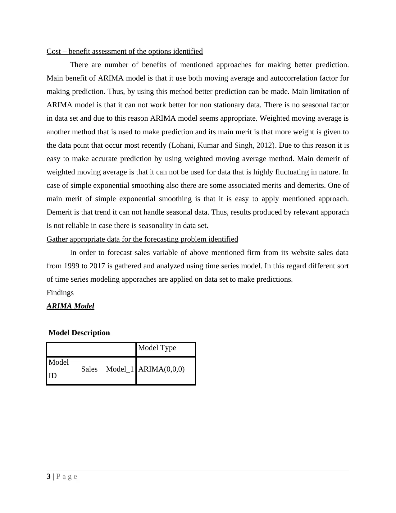
ARIMA Model
Model Description
Model Type
Model
ID Sales Model_1 ARIMA(0,0,0)
3 | P a g e

4 | P a g e

5 | P a g e

Model Fit
Fit
Statistic
Mean S
E
Minim
um
Maxi
mum
Percentile
5 10 25 50 75 90 95
Stationa
ry R-
squared
.012 . .012 .012 .012 .012 .012 .012 .012 .012 .012
R-
squared .012 . .012 .012 .012 .012 .012 .012 .012 .012 .012
6 | P a g e

RMSE 8328.5
07 . 8328.5
07
8328.5
07
8328.5
07
8328.5
07
8328.5
07
8328.5
07
8328.5
07
8328.5
07
8328.5
07
MAPE 87.142 . 87.142 87.142 87.142 87.142 87.142 87.142 87.142 87.142 87.142
MaxAP
E
298.34
5 . 298.34
5
298.34
5
298.34
5
298.34
5
298.34
5
298.34
5
298.34
5
298.34
5
298.34
5
MAE 5398.4
62 . 5398.4
62
5398.4
62
5398.4
62
5398.4
62
5398.4
62
5398.4
62
5398.4
62
5398.4
62
5398.4
62
MaxAE 27887.
048 . 27887.
048
27887.
048
27887.
048
27887.
048
27887.
048
27887.
048
27887.
048
27887.
048
27887.
048
Normal
ized
BIC
18.365 . 18.365 18.365 18.365 18.365 18.365 18.365 18.365 18.365 18.365
Model Statistics
Model Number of
Predictors
Model Fit
statistics
Ljung-Box Q(18) Number of
Outliers
Stationary R-
squared
Statistics DF Sig.
Sales-
Model_1 1 .012 6.329 18 .995 0
7 | P a g e

Interpretation
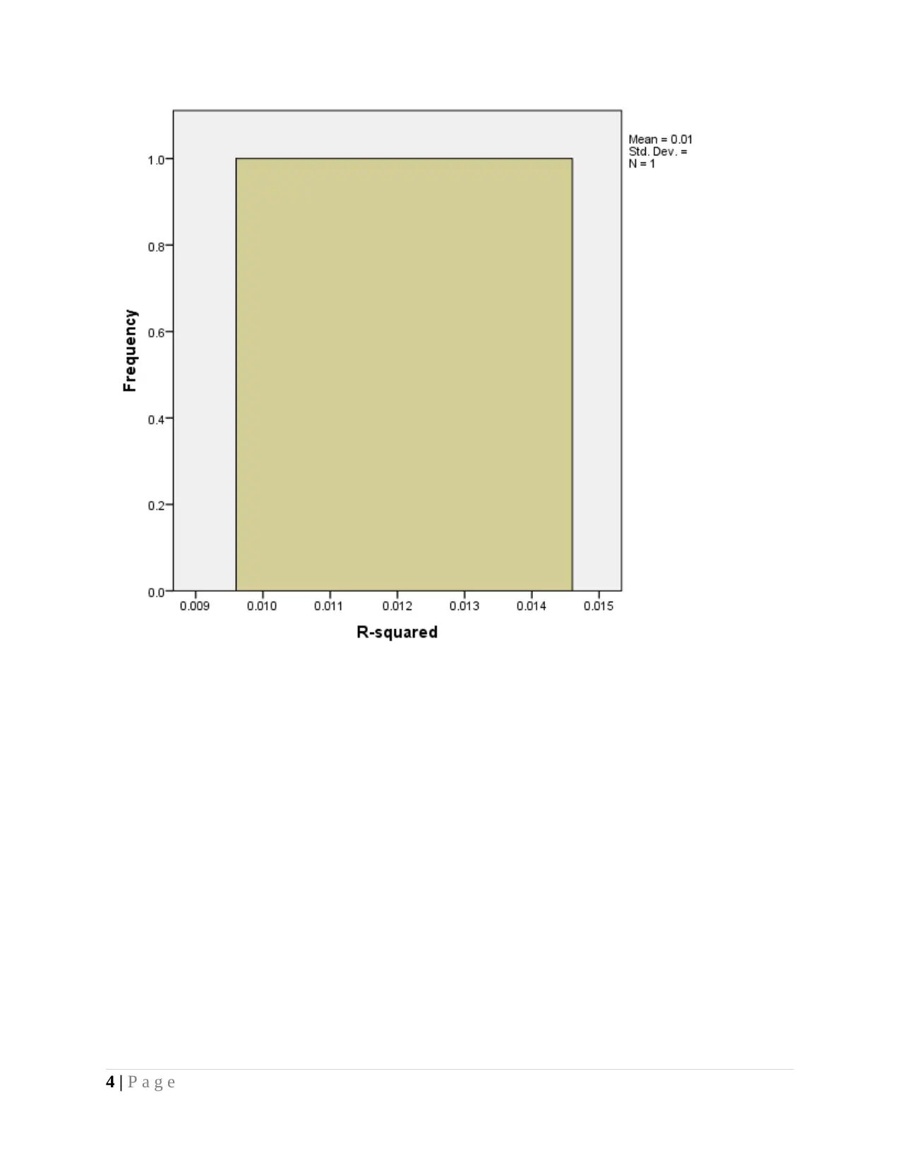
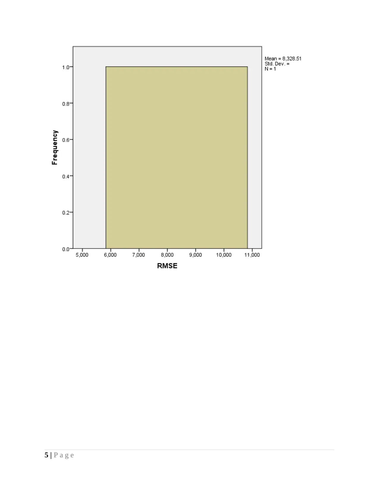
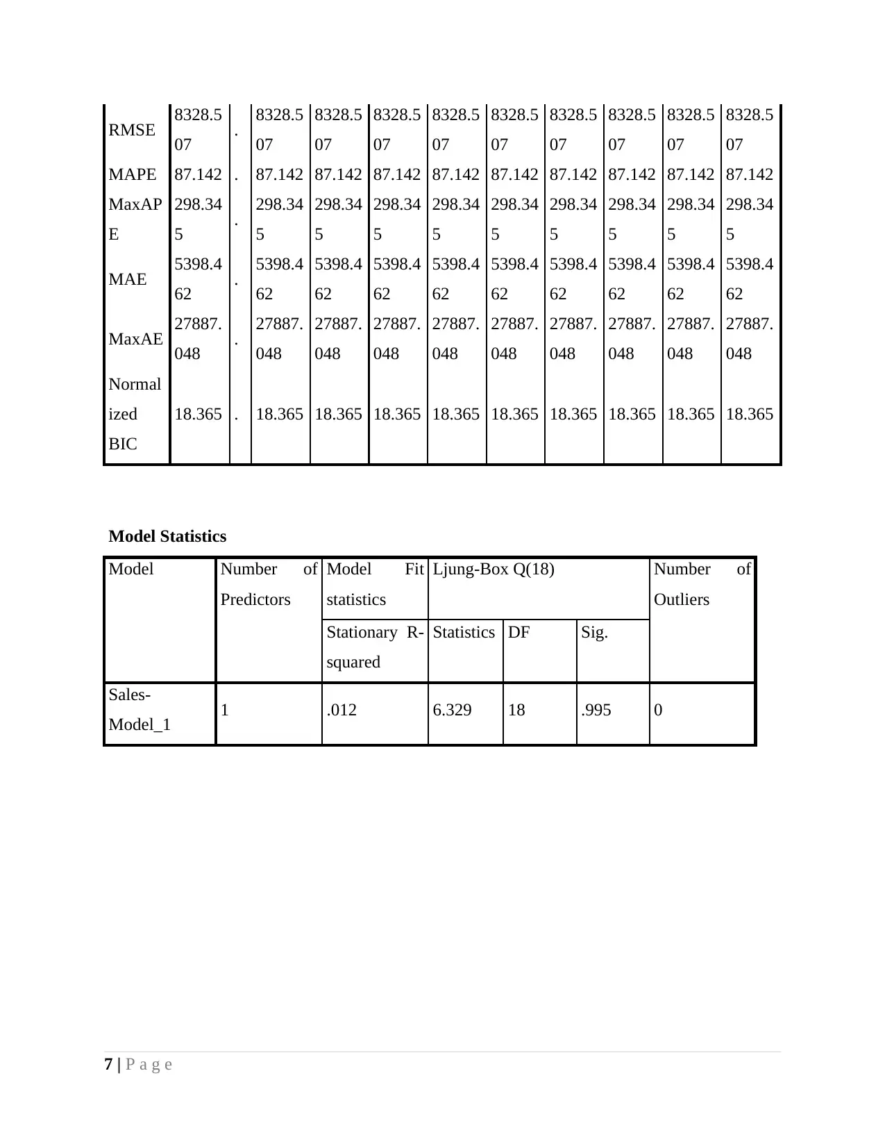
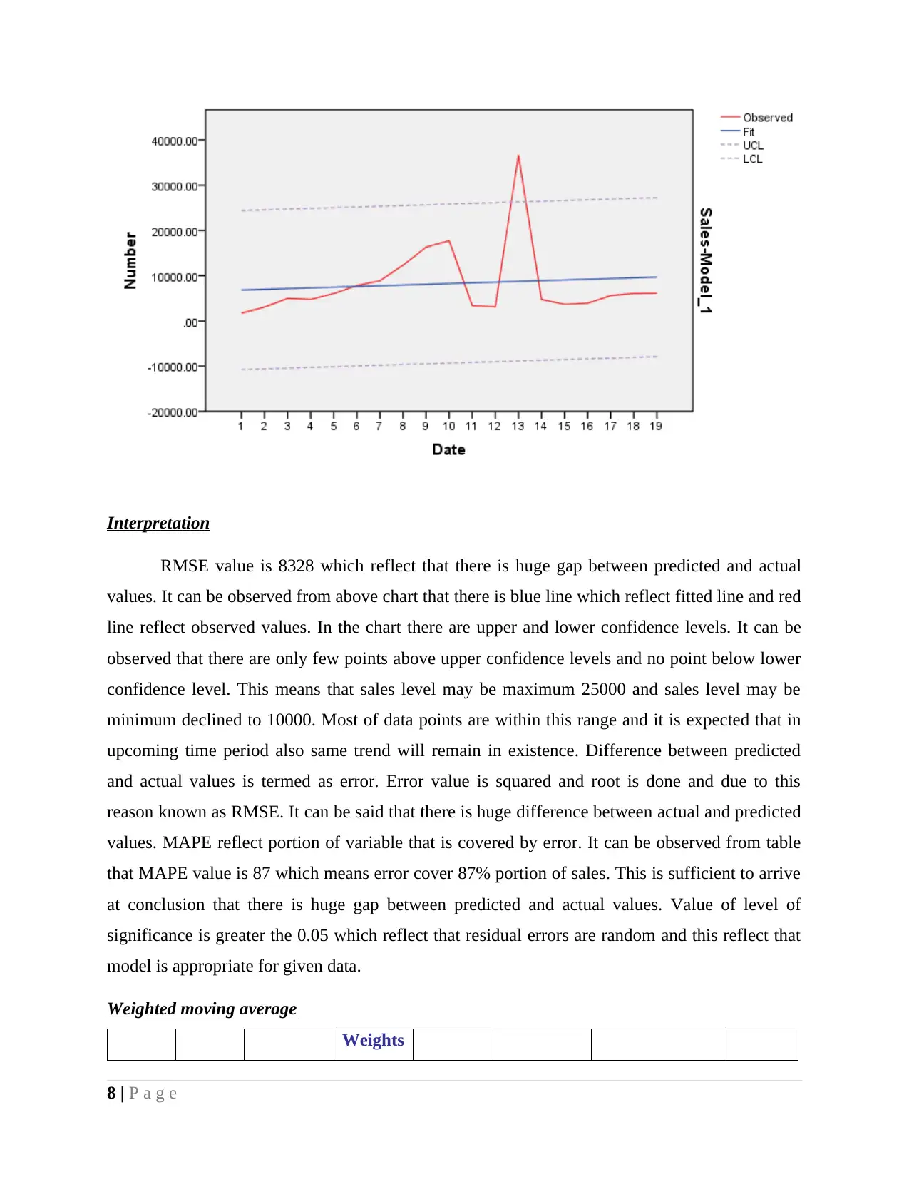
RMSE value is 8328 which reflect that there is huge gap between predicted and actual
values. It can be observed from above chart that there is blue line which reflect fitted line and red
line reflect observed values. In the chart there are upper and lower confidence levels. It can be
observed that there are only few points above upper confidence levels and no point below lower
confidence level. This means that sales level may be maximum 25000 and sales level may be
minimum declined to 10000. Most of data points are within this range and it is expected that in
upcoming time period also same trend will remain in existence. Difference between predicted
and actual values is termed as error. Error value is squared and root is done and due to this
reason known as RMSE. It can be said that there is huge difference between actual and predicted
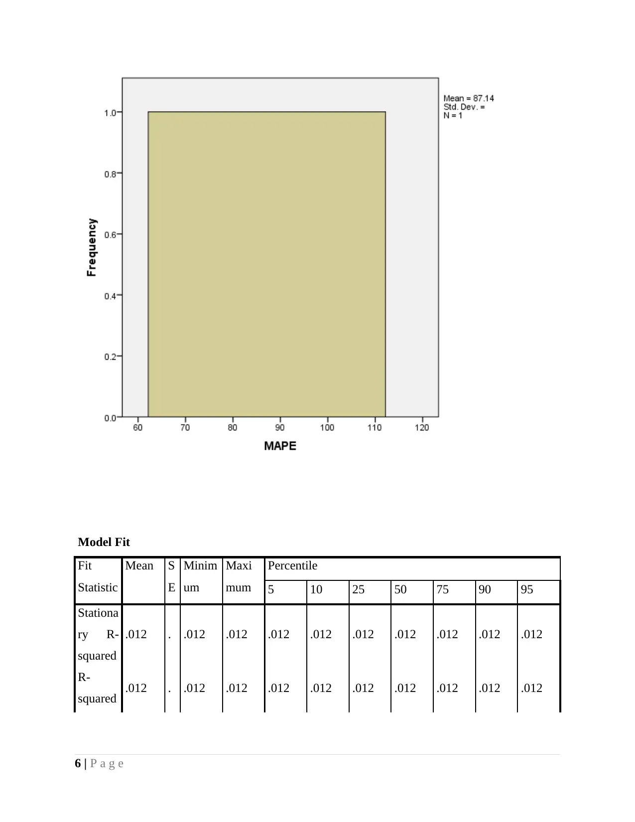
values. MAPE reflect portion of variable that is covered by error. It can be observed from table
that MAPE value is 87 which means error cover 87% portion of sales. This is sufficient to arrive
at conclusion that there is huge gap between predicted and actual values. Value of level of
significance is greater the 0.05 which reflect that residual errors are random and this reflect that
model is appropriate for given data.
Weighted moving average
Weights
8 | P a g e

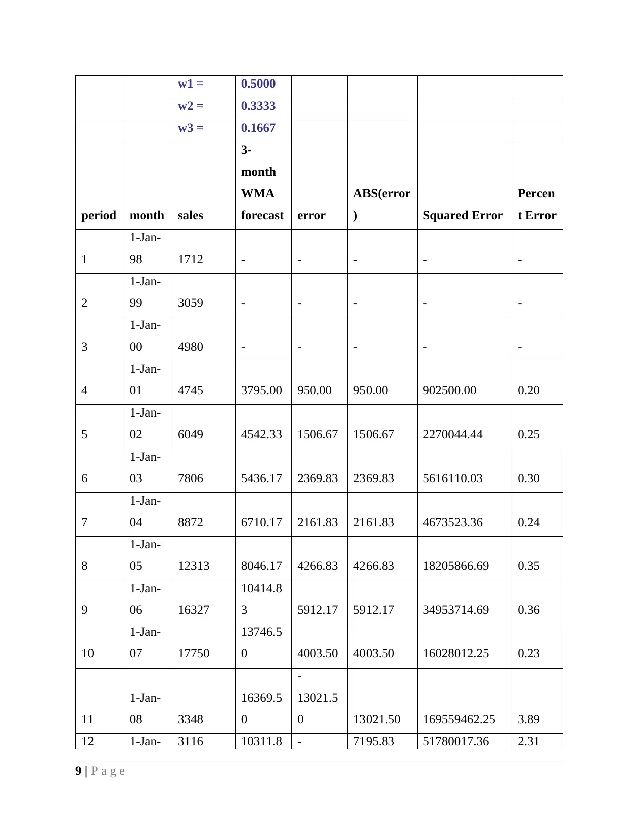
w1 = 0.5000
w2 = 0.3333
w3 = 0.1667
period month sales
3-
month
WMA
forecast error
ABS(error
) Squared Error
Percen
t Error
1
1-Jan-
98 1712 - - - - -
2
1-Jan-
99 3059 - - - - -
3
1-Jan-
00 4980 - - - - -
4
1-Jan-
01 4745 3795.00 950.00 950.00 902500.00 0.20
5
1-Jan-
02 6049 4542.33 1506.67 1506.67 2270044.44 0.25
6
1-Jan-
03 7806 5436.17 2369.83 2369.83 5616110.03 0.30
7
1-Jan-
04 8872 6710.17 2161.83 2161.83 4673523.36 0.24
8
1-Jan-
05 12313 8046.17 4266.83 4266.83 18205866.69 0.35
9
1-Jan-
06 16327
10414.8
3 5912.17 5912.17 34953714.69 0.36
10
1-Jan-
07 17750
13746.5
0 4003.50 4003.50 16028012.25 0.23
11
1-Jan-
08 3348
16369.5
0
-
13021.5
0 13021.50 169559462.25 3.89
12 1-Jan- 3116 10311.8 - 7195.83 51780017.36 2.31
9 | P a g e

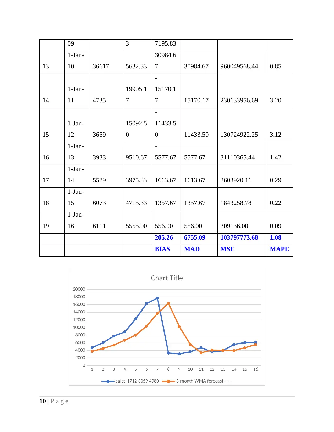
09 3 7195.83
13
1-Jan-
10 36617 5632.33
30984.6
7 30984.67 960049568.44 0.85
14
1-Jan-
11 4735
19905.1
7
-
15170.1
7 15170.17 230133956.69 3.20
15
1-Jan-
12 3659
15092.5
0
-
11433.5
0 11433.50 130724922.25 3.12
16
1-Jan-
13 3933 9510.67
-
5577.67 5577.67 31110365.44 1.42
17
1-Jan-
14 5589 3975.33 1613.67 1613.67 2603920.11 0.29
18
1-Jan-
15 6073 4715.33 1357.67 1357.67 1843258.78 0.22
19
1-Jan-
16 6111 5555.00 556.00 556.00 309136.00 0.09
205.26 6755.09 103797773.68 1.08
BIAS MAD MSE MAPE
1 2 3 4 5 6 7 8 9 10 11 12 13 14 15 16
0
2000
4000
6000
8000
10000
12000
14000
16000
18000
20000
Chart Title
sales 1712 3059 4980 3-month WMA forecast - - -
10 | P a g e