GB513 Business Analytics Unit 4 Assignment Solution - Analysis

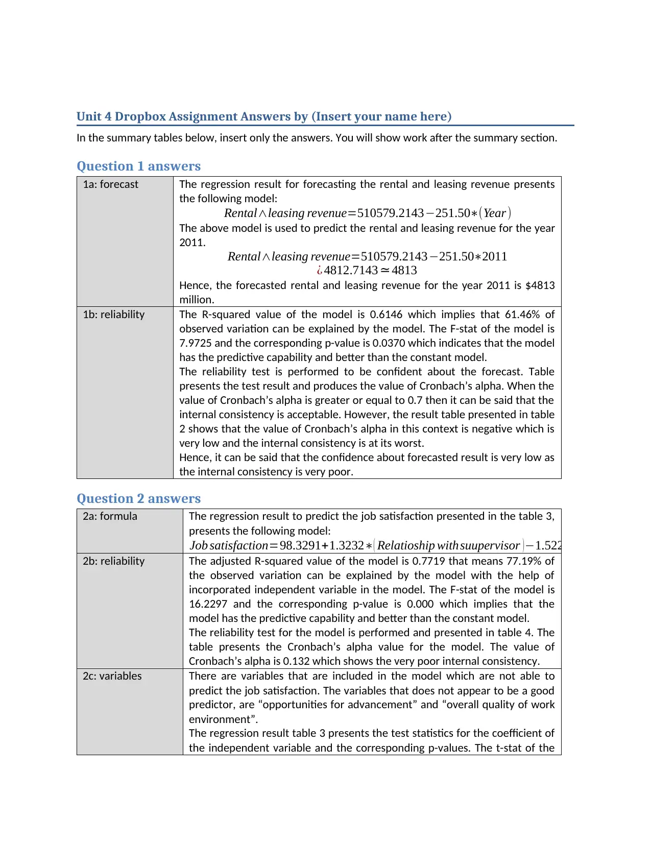
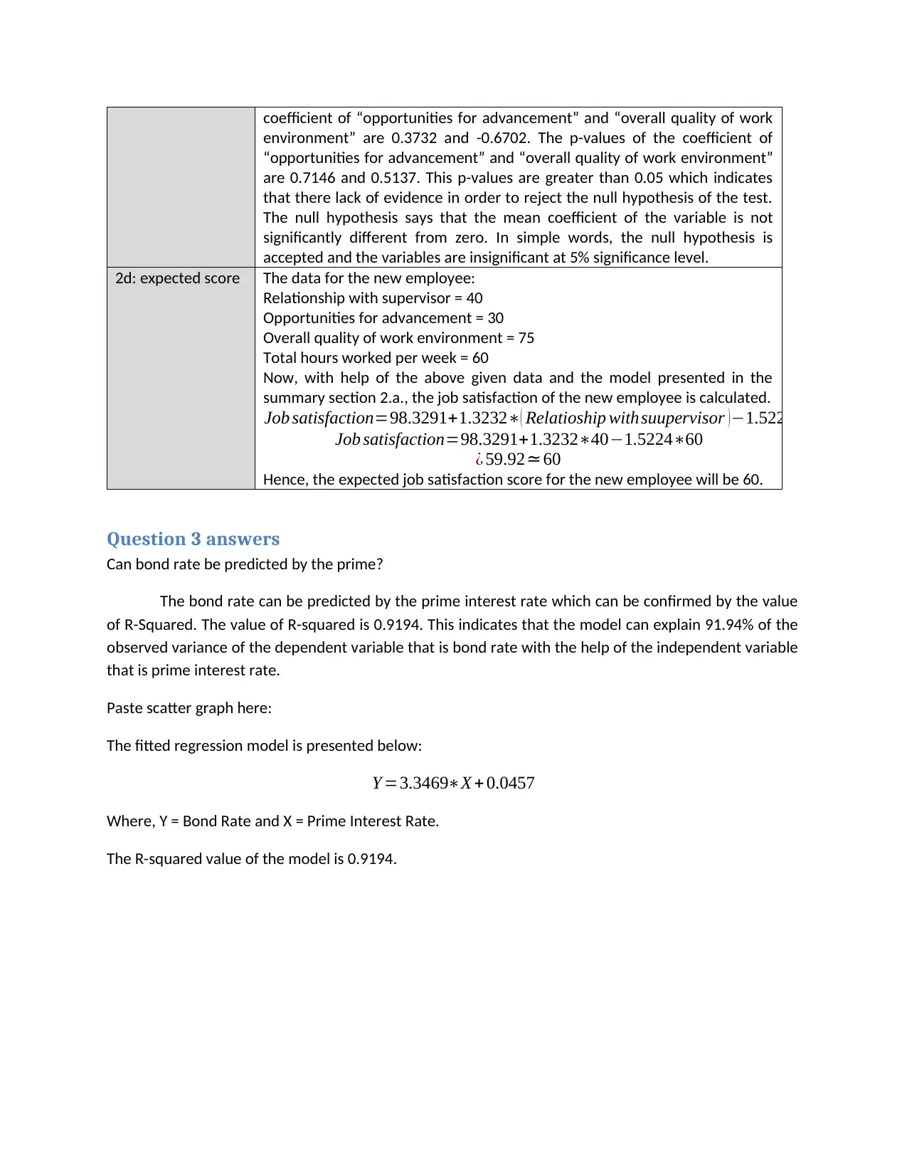
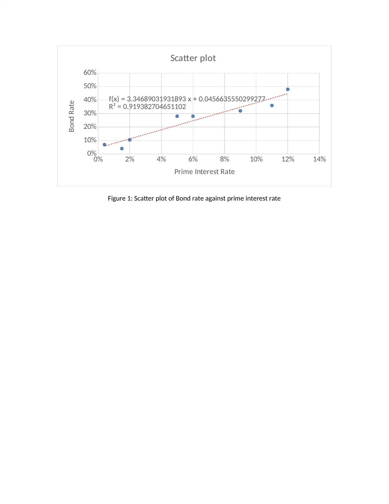
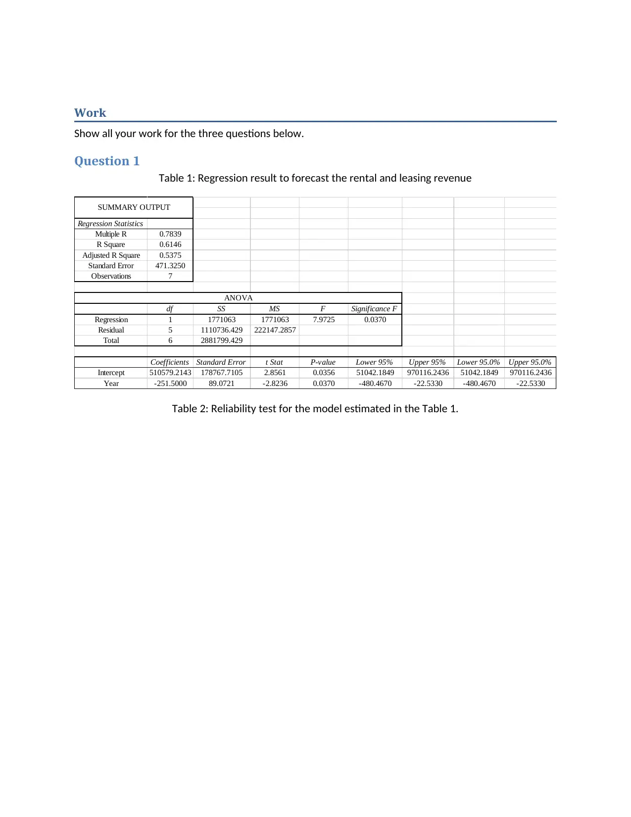
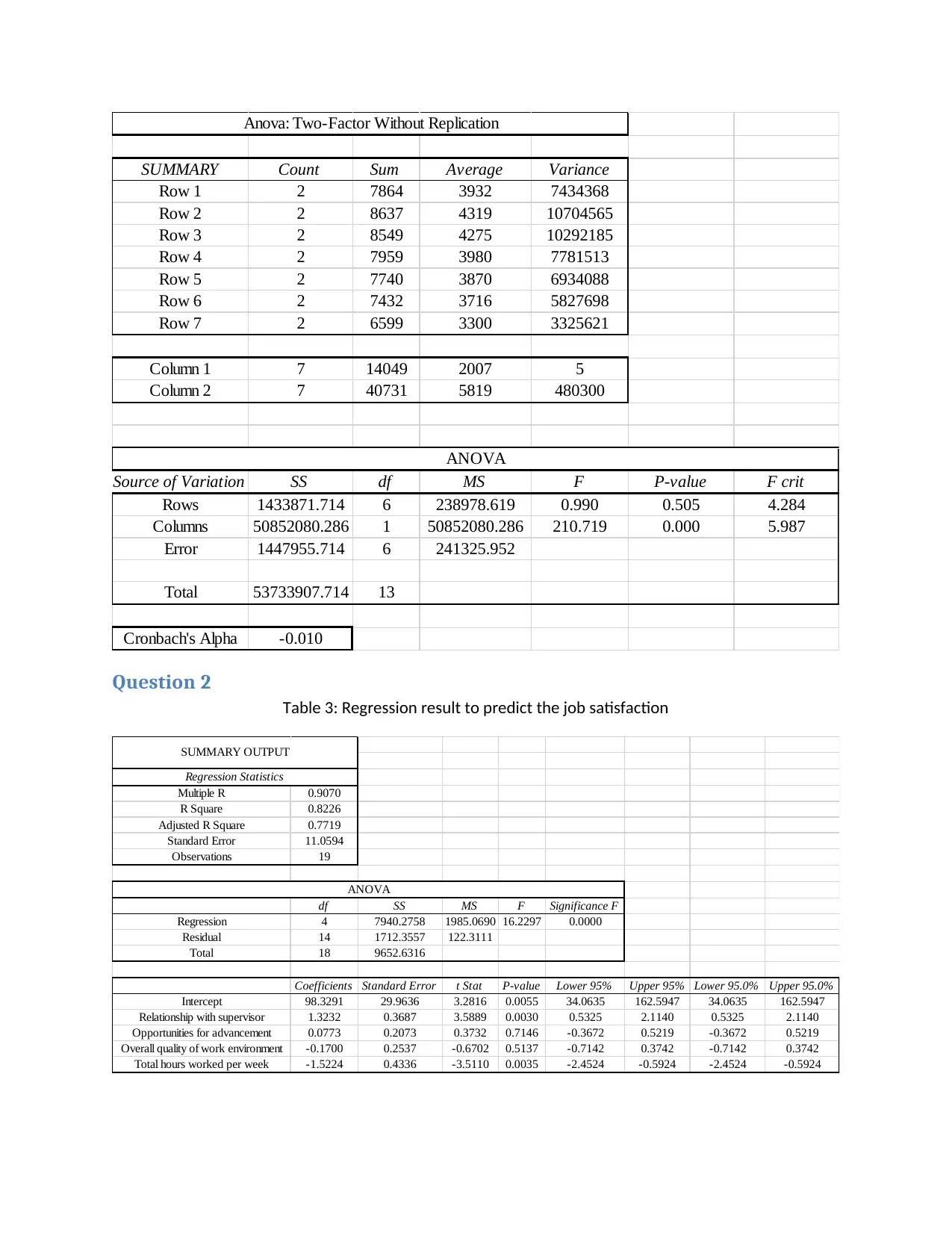
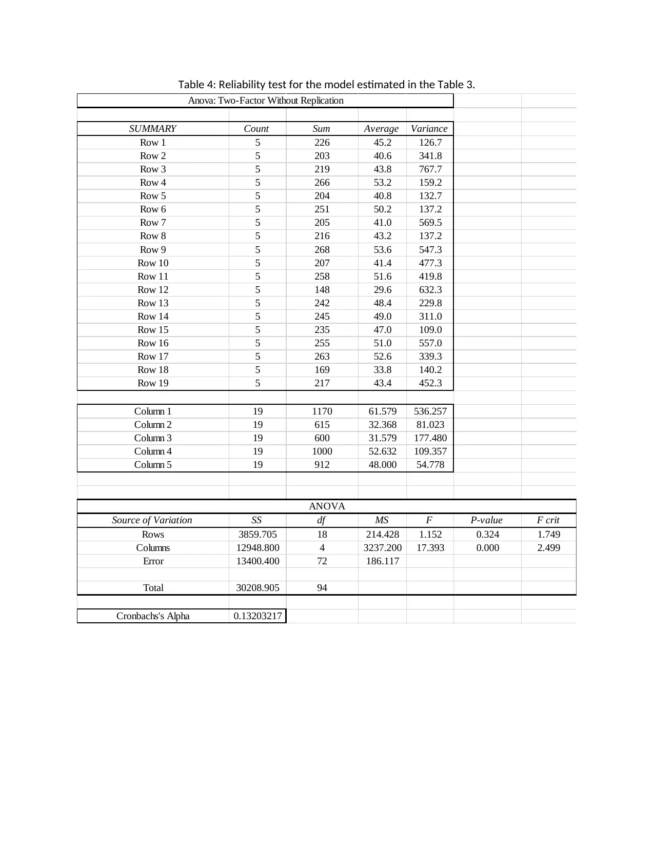
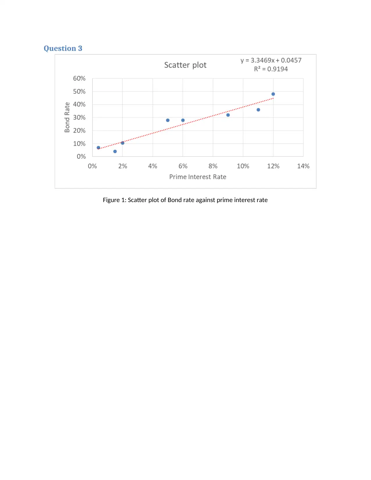
This assignment solution provides answers to three questions from a Business Analytics unit, utilizing Excel for analysis. Question 1 focuses on forecasting rental and leasing revenue using regression analysis, determining the forecast for 2011 and assessing the reliability of the model. Question 2 explores job satisfaction prediction through regression, identifying the formula, assessing reliability, pinpointing insignificant variables, and calculating an expected job satisfaction score for a new employee. Question 3 investigates the relationship between bond rates and prime interest rates using regression and includes a scatter plot. The solution includes the answers, work, regression output tables and explanations for each question.

Unit 4 Dropbox Assignment Answers by (Insert your name here)
In the summary tables below, insert only the answers. You will show work after the summary section.
Question 1 answers
1a: forecast The regression result for forecasting the rental and leasing revenue presents
the following model:
Rental∧leasing revenue=510579.2143−251.50∗(Year)
The above model is used to predict the rental and leasing revenue for the year
2011.
Rental∧leasing revenue=510579.2143−251.50∗2011
¿ 4812.7143 ≃ 4813
Hence, the forecasted rental and leasing revenue for the year 2011 is $4813
million.
1b: reliability The R-squared value of the model is 0.6146 which implies that 61.46% of
observed variation can be explained by the model. The F-stat of the model is
7.9725 and the corresponding p-value is 0.0370 which indicates that the model
has the predictive capability and better than the constant model.
The reliability test is performed to be confident about the forecast. Table
presents the test result and produces the value of Cronbach’s alpha. When the
value of Cronbach’s alpha is greater or equal to 0.7 then it can be said that the
internal consistency is acceptable. However, the result table presented in table
2 shows that the value of Cronbach’s alpha in this context is negative which is
very low and the internal consistency is at its worst.
Hence, it can be said that the confidence about forecasted result is very low as
the internal consistency is very poor.
Question 2 answers
2a: formula The regression result to predict the job satisfaction presented in the table 3,
presents the following model:
Job satisfaction=98.3291+1.3232∗( Relatioship withsuupervisor ) −1.5224∗( Total hours wo
2b: reliability The adjusted R-squared value of the model is 0.7719 that means 77.19% of
the observed variation can be explained by the model with the help of
incorporated independent variable in the model. The F-stat of the model is
16.2297 and the corresponding p-value is 0.000 which implies that the
model has the predictive capability and better than the constant model.
The reliability test for the model is performed and presented in table 4. The
table presents the Cronbach’s alpha value for the model. The value of
Cronbach’s alpha is 0.132 which shows the very poor internal consistency.
2c: variables There are variables that are included in the model which are not able to
predict the job satisfaction. The variables that does not appear to be a good
predictor, are “opportunities for advancement” and “overall quality of work
environment”.
The regression result table 3 presents the test statistics for the coefficient of
the independent variable and the corresponding p-values. The t-stat of the

coefficient of “opportunities for advancement” and “overall quality of work
environment” are 0.3732 and -0.6702. The p-values of the coefficient of
“opportunities for advancement” and “overall quality of work environment”
are 0.7146 and 0.5137. This p-values are greater than 0.05 which indicates
that there lack of evidence in order to reject the null hypothesis of the test.
The null hypothesis says that the mean coefficient of the variable is not
significantly different from zero. In simple words, the null hypothesis is
accepted and the variables are insignificant at 5% significance level.
2d: expected score The data for the new employee:
Relationship with supervisor = 40
Opportunities for advancement = 30
Overall quality of work environment = 75
Total hours worked per week = 60
Now, with help of the above given data and the model presented in the
summary section 2.a., the job satisfaction of the new employee is calculated.
Job satisfaction=98.3291+1.3232∗( Relatioship withsuupervisor ) −1.5224∗( Total hours wo
Job satisfaction=98.3291+1.3232∗40−1.5224∗60
¿ 59.92≃60
Hence, the expected job satisfaction score for the new employee will be 60.
Question 3 answers
Can bond rate be predicted by the prime?
The bond rate can be predicted by the prime interest rate which can be confirmed by the value
of R-Squared. The value of R-squared is 0.9194. This indicates that the model can explain 91.94% of the
observed variance of the dependent variable that is bond rate with the help of the independent variable
that is prime interest rate.
Paste scatter graph here:
The fitted regression model is presented below:
Y =3.3469∗X + 0.0457
Where, Y = Bond Rate and X = Prime Interest Rate.
The R-squared value of the model is 0.9194.

0% 2% 4% 6% 8% 10% 12% 14%
0%
10%
20%
30%
40%
50%
60%
f(x) = 3.34689031931893 x + 0.0456635550299277
R² = 0.919382704651102
Scatter plot
Prime Interest Rate
Bond Rate
Figure 1: Scatter plot of Bond rate against prime interest rate

Work
Show all your work for the three questions below.
Question 1
Table 1: Regression result to forecast the rental and leasing revenue
Regression Statistics
Multiple R 0.7839
R Square 0.6146
Adjusted R Square 0.5375
Standard Error 471.3250
Observations 7
df SS MS F Significance F
Regression 1 1771063 1771063 7.9725 0.0370
Residual 5 1110736.429 222147.2857
Total 6 2881799.429
Coefficients Standard Error t Stat P-value Lower 95% Upper 95% Lower 95.0% Upper 95.0%
Intercept 510579.2143 178767.7105 2.8561 0.0356 51042.1849 970116.2436 51042.1849 970116.2436
Year -251.5000 89.0721 -2.8236 0.0370 -480.4670 -22.5330 -480.4670 -22.5330
SUMMARY OUTPUT
ANOVA
Table 2: Reliability test for the model estimated in the Table 1.

SUMMARY Count Sum Average Variance
Row 1 2 7864 3932 7434368
Row 2 2 8637 4319 10704565
Row 3 2 8549 4275 10292185
Row 4 2 7959 3980 7781513
Row 5 2 7740 3870 6934088
Row 6 2 7432 3716 5827698
Row 7 2 6599 3300 3325621
Column 1 7 14049 2007 5
Column 2 7 40731 5819 480300
Source of Variation SS df MS F P-value F crit
Rows 1433871.714 6 238978.619 0.990 0.505 4.284
Columns 50852080.286 1 50852080.286 210.719 0.000 5.987
Error 1447955.714 6 241325.952
Total 53733907.714 13
Cronbach's Alpha -0.010
Anova: Two-Factor Without Replication
ANOVA
Question 2
Table 3: Regression result to predict the job satisfaction
Multiple R 0.9070
R Square 0.8226
Adjusted R Square 0.7719
Standard Error 11.0594
Observations 19
df SS MS F Significance F
Regression 4 7940.2758 1985.0690 16.2297 0.0000
Residual 14 1712.3557 122.3111
Total 18 9652.6316
Coefficients Standard Error t Stat P-value Lower 95% Upper 95% Lower 95.0% Upper 95.0%
Intercept 98.3291 29.9636 3.2816 0.0055 34.0635 162.5947 34.0635 162.5947
Relationship with supervisor 1.3232 0.3687 3.5889 0.0030 0.5325 2.1140 0.5325 2.1140
Opportunities for advancement 0.0773 0.2073 0.3732 0.7146 -0.3672 0.5219 -0.3672 0.5219
Overall quality of work environment -0.1700 0.2537 -0.6702 0.5137 -0.7142 0.3742 -0.7142 0.3742
Total hours worked per week -1.5224 0.4336 -3.5110 0.0035 -2.4524 -0.5924 -2.4524 -0.5924
SUMMARY OUTPUT
ANOVA
Regression Statistics

Table 4: Reliability test for the model estimated in the Table 3.
SUMMARY Count Sum Average Variance
Row 1 5 226 45.2 126.7
Row 2 5 203 40.6 341.8
Row 3 5 219 43.8 767.7
Row 4 5 266 53.2 159.2
Row 5 5 204 40.8 132.7
Row 6 5 251 50.2 137.2
Row 7 5 205 41.0 569.5
Row 8 5 216 43.2 137.2
Row 9 5 268 53.6 547.3
Row 10 5 207 41.4 477.3
Row 11 5 258 51.6 419.8
Row 12 5 148 29.6 632.3
Row 13 5 242 48.4 229.8
Row 14 5 245 49.0 311.0
Row 15 5 235 47.0 109.0
Row 16 5 255 51.0 557.0
Row 17 5 263 52.6 339.3
Row 18 5 169 33.8 140.2
Row 19 5 217 43.4 452.3
Column 1 19 1170 61.579 536.257
Column 2 19 615 32.368 81.023
Column 3 19 600 31.579 177.480
Column 4 19 1000 52.632 109.357
Column 5 19 912 48.000 54.778
Source of Variation SS df MS F P-value F crit
Rows 3859.705 18 214.428 1.152 0.324 1.749
Columns 12948.800 4 3237.200 17.393 0.000 2.499
Error 13400.400 72 186.117
Total 30208.905 94
Cronbachs's Alpha 0.13203217
Anova: Two-Factor Without Replication
ANOVA

Question 3
Figure 1: Scatter plot of Bond rate against prime interest rate