Gender Pay Gap in Australia: Microeconomics Report and Analysis
VerifiedAdded on 2021/06/17
|19
|3123
|62
Report
AI Summary
This report presents an analysis of the gender pay gap among highly educated individuals in Australia, focusing on those with graduate degrees. The study utilizes data from the Australian Household Survey of 2015-2016, employing OLS estimators to assess wage differentials. The report examines various factors, including age, gender, marital status, and occupation, to determine their impact on wages. The methodology involves initial model development, testing assumptions such as multicollinearity and normality, and refining the model to address heteroskedasticity. Results indicate little to no gender pay gap among the highly educated population, though limitations exist due to the use of OLS estimators with complex panel data. The report provides detailed data summaries, including descriptive statistics and scatter plots, and concludes with an overview of the findings and potential areas for further research. Tables and figures are used to illustrate the findings of the research.
Question 2: Microeconomics – Wages
Executive Summary
The given report is an estimation of the gender pay gap among the highly educated
population of Australia i.e. the population that has at least a graduate degree. Gender pay
gap is a hotly debated topic worldwide with almost every field of work showing a Gender
Pay Gap. This report has observed little to no gender pay gap among the highly educated
population in Australia. However, there might be shortcomings to these results as OLS
estimators are very weak predictors of variables in complex Panel Data.
Paraphrase This Document
Need a fresh take? Get an instant paraphrase of this document with our AI Paraphraser
Contents
1. Introduction................................................................................................................................... 1
2. Data............................................................................................................................................... 1
2.1. Data Description.................................................................................................................... 1
2.2. Data Summary....................................................................................................................... 2
3. Methodology................................................................................................................................. 8
3.1. Initial Model........................................................................................................................... 8
3.2. Testing Assumptions..............................................................................................................8
3.3. Final Model and Estimation Technique.................................................................................. 8
4. Results......................................................................................................................................... 10
5. Conclusion................................................................................................................................... 12
6. Appendix...................................................................................................................................... 13
7. References................................................................................................................................... 13
Figure 1 Summary Statistics for the Industry of the Main Job of the Respondent = Accommodation
and Food Services,................................................................................................................................. 2
Figure 2 Scatter Plot of Wages Earned Per Hour Against Age................................................................6
Figure 3 Scatter Plot of Wages Earned Per Hour Against Number of Hours worked per week..............7
Table 1 Variables’ Name, Description and Type/Units..........................................................................1
Table 2 Summary Statistics for Log of Wages, female respondents, respondents who are working and
married, the total number of children in the household, and the square of the age of the respondent
...............................................................................................................................................................2
Table 31 Figure 1 Summary Statistics for the Industry of the Main Job of the Respondent =
Accommodation and Food Services,......................................................................................................2
Table 4 Summary Statistics for the Industry of the Main Job of the Respondent = Accommodation
and Food Services; Administrative and Support services, ; Agriculture, Forestry and Fishing..............3
Table 5 Summary Statistics for the Industry of the Main Job of the Respondent = Arts and Recreation
Services; or Construction; or Education and Training............................................................................3
Table 6 Summary Statistics for the Industry of the Main Job of the Respondent = Electricity, Gas,
Water and Waste Services; or Financial and Insurance Services or Health Care and Social Assistance.3
Table 7 Summary Statistics for the Industry of the Main Job of the Respondent = Information Media
and Telecommunications; or Manufacturing; or Mining.......................................................................4
Table 8 Summary Statistics for the Industry of the Main Job of the Respondent = Other Services; or
Professional, Scientific and Technical Services; Public Administration and Safety or Rental, Hiring and
Real Estate Services...............................................................................................................................4
Table 9 Summary Statistics for the Industry of the Main Job of the Respondent = Retail Trade; or
Transport, Postal and Warehousing; or Wholesale Trade.....................................................................4
Table 10 Summary Statistics for the Occupation of the Main Job of the Respondent = Community and
Personal Service Workers; or Labourers; or Machinery Operators and Drivers....................................5
Table 11 Summary Statistics for the Occupation of the Main Job of the Respondent = Machinery
Operators and Drivers; or Professionals................................................................................................5
Table 12 Summary Statistics for the Occupation of the Main Job of the Respondent = Sales Workers;
or Technicians and Trade Workers........................................................................................................ 6
Table 13 Scatter Plot (Years_with_children_in_the Household) and (ln_wages)..................................9
Table 15 OLS Estimates of Model A..................................................................................................... 11
Table 16 OLS Estimates of Model B..................................................................................................... 11
Table 17 Mean Comparison between Independent Variable for Male and Female Workers.............11
Table 18 Normality Test (Jarque –Bera Test).......................................................................................13
⊘ This is a preview!⊘
Do you want full access?
Subscribe today to unlock all pages.
Trusted by 1+ million students worldwide
1. Introduction
OLS Estimators or regressions are used to make forecasts to understand the importance of a given
variable in determining a dependent variable. Gender parity is a hotly debated topic currently as
Australian industries too seem to have a gender pay gap. (Organization for Economic Co-operation
and Development, 2017). This report is an attempt to analyse the gender pay gap among the highly
educated population (i,e population that has at least a graduate degree). In order to do so, OLS
estimation has been used on a sample collected from the Household Survey of Australia, 2015-2016.
(Australian Bureau Of Statistics, 2017)
2. Data
The Data for taken from the Australian Household Survey for 205-2016. (Australian Bureau Of
Statistics, 2017)This Panel data survey respondents on a variety of demographic indicators such as
age, education, wage, number of house works. The given data is a sample from this database. The
data contains sample for only those workers who have at least a graduate degree. The data for
cleaned before analyses, in order to remove outliers. Accordingly, the top 1% earners i,e those
earning more than 183.03 AUD and the bottom 1% earner i.e. those earning less than 7.61AUD were
removed as observations. Similarly, average wages are not a good statistic to consider since the
wage differentials can be a result of the cost of living in a region. Hence, the log of wages or ln wages
has been used as dependent variable in the OLS estimator. The log of a variable considers the
elasticity of a variable, given a change in another variable, instead of the absolute value.
(Wooldridge, 2015)
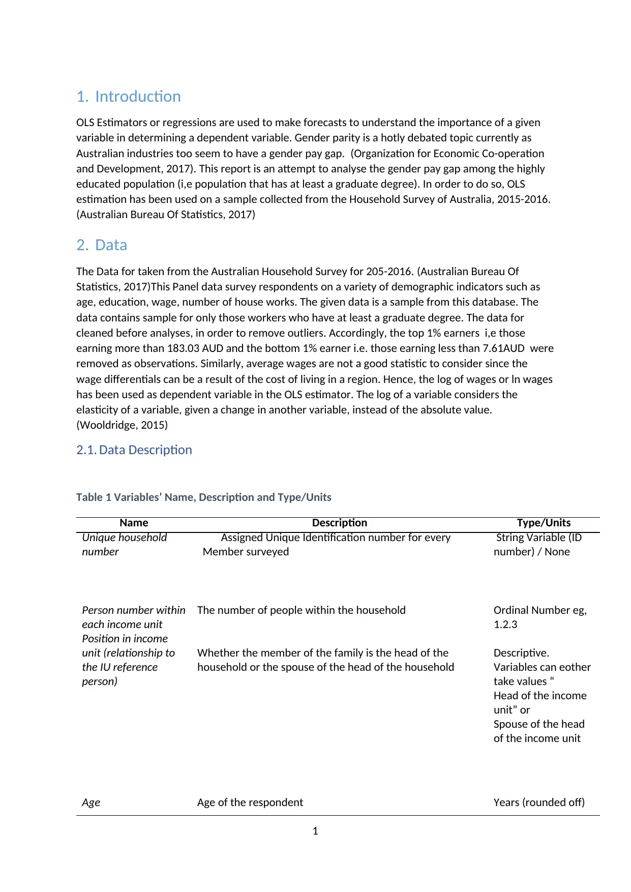
2.1. Data Description
Table 1 Variables’ Name, Description and Type/Units
Name Description Type/Units
Unique household
number
Assigned Unique Identification number for every
Member surveyed
String Variable (ID
number) / None
Person number within
each income unit
Position in income
unit (relationship to
the IU reference
person)
The number of people within the household
Whether the member of the family is the head of the
household or the spouse of the head of the household
Ordinal Number eg,
1.2.3
Descriptive.
Variables can eother
take values “
Head of the income
unit” or
Spouse of the head
of the income unit
Age Age of the respondent Years (rounded off)
1
OLS Estimators or regressions are used to make forecasts to understand the importance of a given
variable in determining a dependent variable. Gender parity is a hotly debated topic currently as
Australian industries too seem to have a gender pay gap. (Organization for Economic Co-operation
and Development, 2017). This report is an attempt to analyse the gender pay gap among the highly
educated population (i,e population that has at least a graduate degree). In order to do so, OLS
estimation has been used on a sample collected from the Household Survey of Australia, 2015-2016.
(Australian Bureau Of Statistics, 2017)
2. Data
The Data for taken from the Australian Household Survey for 205-2016. (Australian Bureau Of
Statistics, 2017)This Panel data survey respondents on a variety of demographic indicators such as
age, education, wage, number of house works. The given data is a sample from this database. The
data contains sample for only those workers who have at least a graduate degree. The data for
cleaned before analyses, in order to remove outliers. Accordingly, the top 1% earners i,e those
earning more than 183.03 AUD and the bottom 1% earner i.e. those earning less than 7.61AUD were
removed as observations. Similarly, average wages are not a good statistic to consider since the
wage differentials can be a result of the cost of living in a region. Hence, the log of wages or ln wages
has been used as dependent variable in the OLS estimator. The log of a variable considers the
elasticity of a variable, given a change in another variable, instead of the absolute value.
(Wooldridge, 2015)
2.1. Data Description
Table 1 Variables’ Name, Description and Type/Units
Name Description Type/Units
Unique household
number
Assigned Unique Identification number for every
Member surveyed
String Variable (ID
number) / None
Person number within
each income unit
Position in income
unit (relationship to
the IU reference
person)
The number of people within the household
Whether the member of the family is the head of the
household or the spouse of the head of the household
Ordinal Number eg,
1.2.3
Descriptive.
Variables can eother
take values “
Head of the income
unit” or
Spouse of the head
of the income unit
Age Age of the respondent Years (rounded off)
1
Paraphrase This Document
Need a fresh take? Get an instant paraphrase of this document with our AI Paraphraser
Wage Hourly wage earned by the person Dollars
Female Indicates whether the person is female or not 1,0 (dummy
variable)
Ft/pt Indicates whether the person is employed full time or part
time.
1,0 (dummy
variable)
Ind Indicates the industry that a person is employed in, from a
pre-drawn list of industries
Categorical string
data, pre selected
categories
OCC Indicates the occupation that the person is employed in Categorical string
data, pre selected
categories
2.2. Data Summary
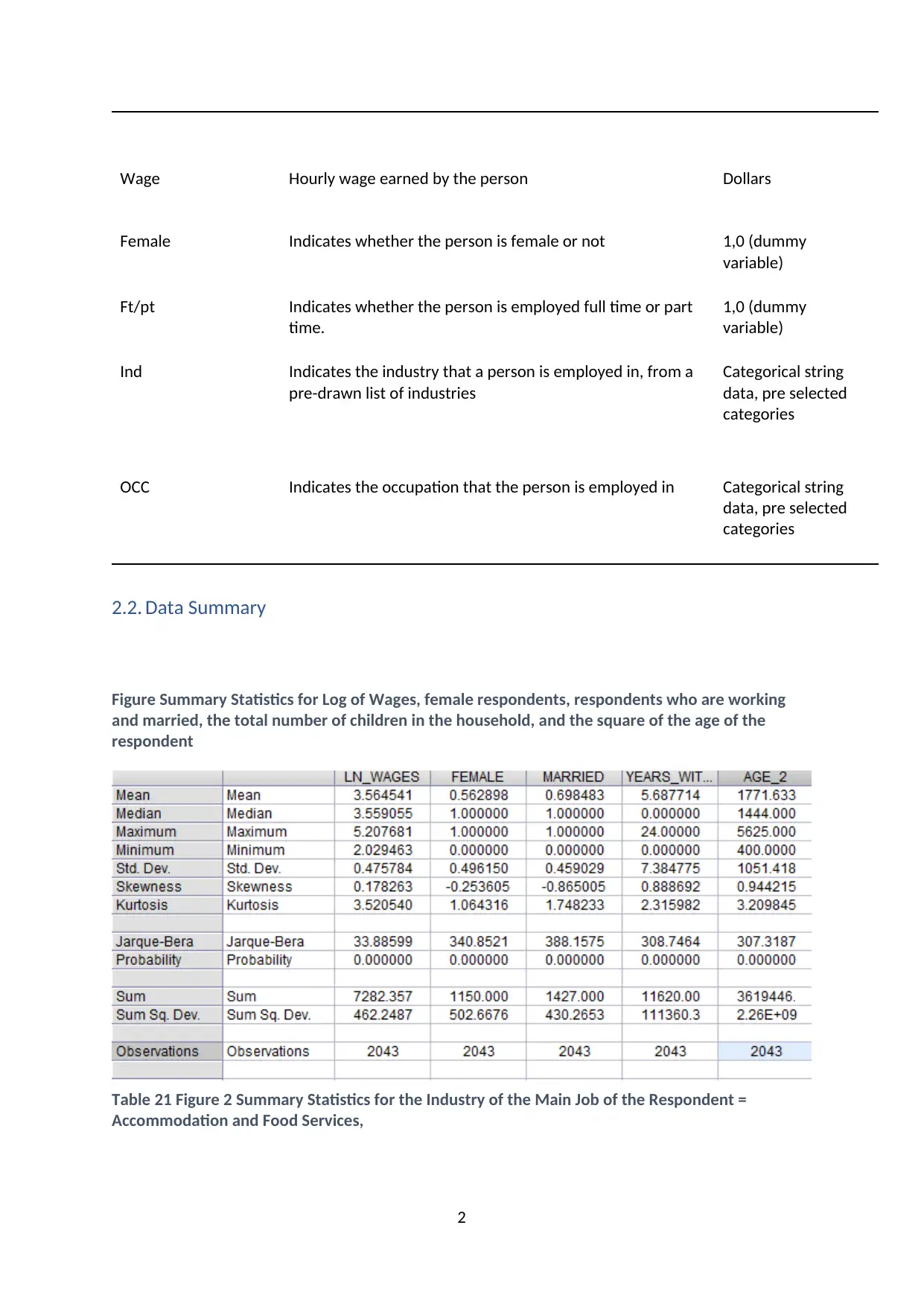
Figure Summary Statistics for Log of Wages, female respondents, respondents who are working
and married, the total number of children in the household, and the square of the age of the
respondent
Table 21 Figure 2 Summary Statistics for the Industry of the Main Job of the Respondent =
Accommodation and Food Services,
2
Female Indicates whether the person is female or not 1,0 (dummy
variable)
Ft/pt Indicates whether the person is employed full time or part
time.
1,0 (dummy
variable)
Ind Indicates the industry that a person is employed in, from a
pre-drawn list of industries
Categorical string
data, pre selected
categories
OCC Indicates the occupation that the person is employed in Categorical string
data, pre selected
categories
2.2. Data Summary
Figure Summary Statistics for Log of Wages, female respondents, respondents who are working
and married, the total number of children in the household, and the square of the age of the
respondent
Table 21 Figure 2 Summary Statistics for the Industry of the Main Job of the Respondent =
Accommodation and Food Services,
2
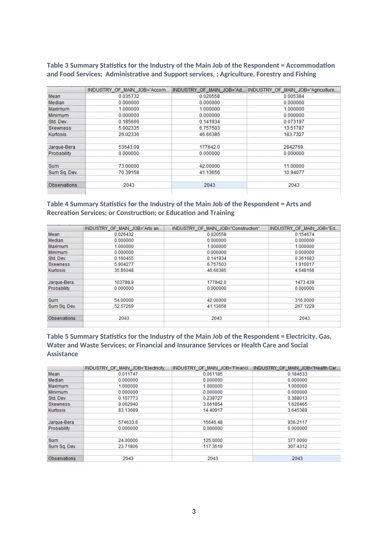
Table 3 Summary Statistics for the Industry of the Main Job of the Respondent = Accommodation
and Food Services; Administrative and Support services, ; Agriculture, Forestry and Fishing
Table 4 Summary Statistics for the Industry of the Main Job of the Respondent = Arts and
Recreation Services; or Construction; or Education and Training
Table 5 Summary Statistics for the Industry of the Main Job of the Respondent = Electricity, Gas,
Water and Waste Services; or Financial and Insurance Services or Health Care and Social
Assistance
3
⊘ This is a preview!⊘
Do you want full access?
Subscribe today to unlock all pages.
Trusted by 1+ million students worldwide

Table 6 Summary Statistics for the Industry of the Main Job of the Respondent = Information
Media and Telecommunications; or Manufacturing; or Mining
Table 7 Summary Statistics for the Industry of the Main Job of the Respondent = Other Services;
or Professional, Scientific and Technical Services; Public Administration and Safety or Rental,
Hiring and Real Estate Services
Table 8 Summary Statistics for the Industry of the Main Job of the Respondent = Retail Trade; or
Transport, Postal and Warehousing; or Wholesale Trade
4
Paraphrase This Document
Need a fresh take? Get an instant paraphrase of this document with our AI Paraphraser
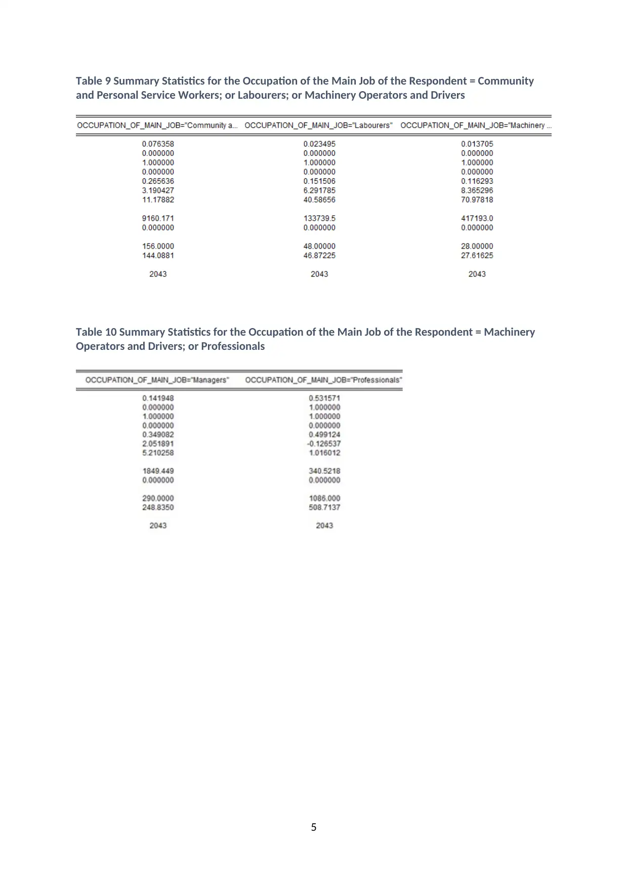
Table 9 Summary Statistics for the Occupation of the Main Job of the Respondent = Community
and Personal Service Workers; or Labourers; or Machinery Operators and Drivers
Table 10 Summary Statistics for the Occupation of the Main Job of the Respondent = Machinery
Operators and Drivers; or Professionals
5
and Personal Service Workers; or Labourers; or Machinery Operators and Drivers
Table 10 Summary Statistics for the Occupation of the Main Job of the Respondent = Machinery
Operators and Drivers; or Professionals
5
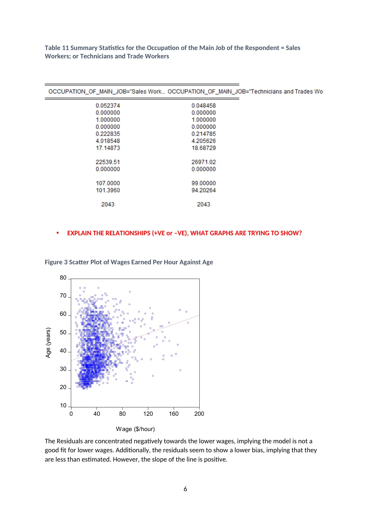
Table 11 Summary Statistics for the Occupation of the Main Job of the Respondent = Sales
Workers; or Technicians and Trade Workers
EXPLAIN THE RELATIONSHIPS (+VE or –VE), WHAT GRAPHS ARE TRYING TO SHOW?
Figure 3 Scatter Plot of Wages Earned Per Hour Against Age
10
20
30
40
50
60
70
80
0 40 80 120 160 200
Wage ($/hour)
Age (years)
The Residuals are concentrated negatively towards the lower wages, implying the model is not a
good fit for lower wages. Additionally, the residuals seem to show a lower bias, implying that they
are less than estimated. However, the slope of the line is positive.
6
⊘ This is a preview!⊘
Do you want full access?
Subscribe today to unlock all pages.
Trusted by 1+ million students worldwide

Figure 4 Scatter Plot of Wages Earned Per Hour Against Number of Hours worked per week
0
10
20
30
40
50
60
70
0 40 80 120 160 200
Wage ($/hour)
Hours (hour/week)
The regression line is almost parallel with a very light downward trend. The Residuals are
concentrated negatively towards the lower wages, implying the model is not a good fit for lower
wages. The model is a better fit when the wages are higher.
7
Paraphrase This Document
Need a fresh take? Get an instant paraphrase of this document with our AI Paraphraser
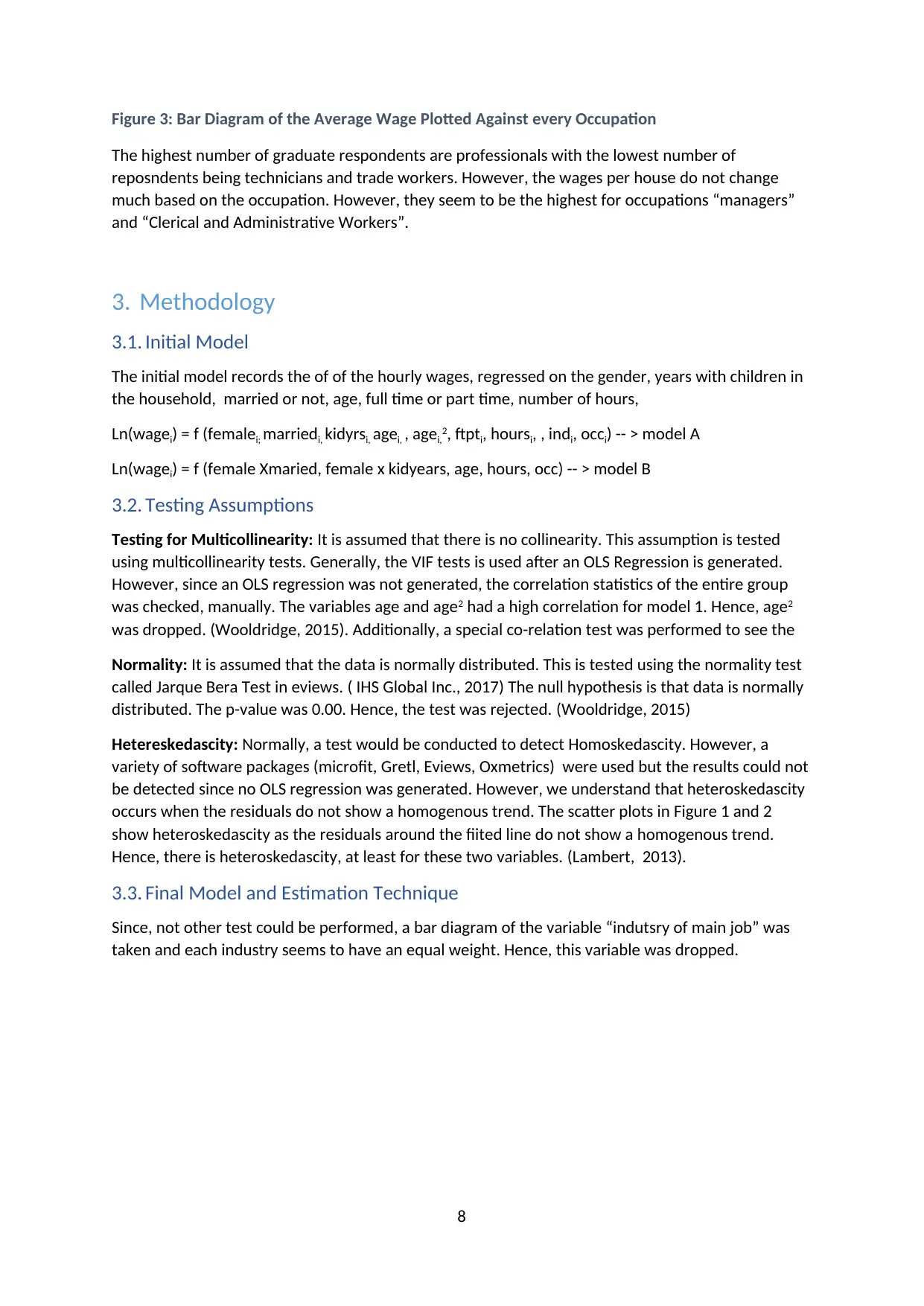
Figure 3: Bar Diagram of the Average Wage Plotted Against every Occupation
The highest number of graduate respondents are professionals with the lowest number of
reposndents being technicians and trade workers. However, the wages per house do not change
much based on the occupation. However, they seem to be the highest for occupations “managers”
and “Clerical and Administrative Workers”.
3. Methodology
3.1. Initial Model
The initial model records the of of the hourly wages, regressed on the gender, years with children in
the household, married or not, age, full time or part time, number of hours,
Ln(wagei) = f (femalei; marriedi, kidyrsi, agei, , agei,2, ftpti, hoursi, , indi, occi) -- > model A
Ln(wagei) = f (female Xmaried, female x kidyears, age, hours, occ) -- > model B
3.2. Testing Assumptions
Testing for Multicollinearity: It is assumed that there is no collinearity. This assumption is tested
using multicollinearity tests. Generally, the VIF tests is used after an OLS Regression is generated.
However, since an OLS regression was not generated, the correlation statistics of the entire group
was checked, manually. The variables age and age2 had a high correlation for model 1. Hence, age2
was dropped. (Wooldridge, 2015). Additionally, a special co-relation test was performed to see the
Normality: It is assumed that the data is normally distributed. This is tested using the normality test
called Jarque Bera Test in eviews. ( IHS Global Inc., 2017) The null hypothesis is that data is normally
distributed. The p-value was 0.00. Hence, the test was rejected. (Wooldridge, 2015)
Hetereskedascity: Normally, a test would be conducted to detect Homoskedascity. However, a
variety of software packages (microfit, Gretl, Eviews, Oxmetrics) were used but the results could not
be detected since no OLS regression was generated. However, we understand that heteroskedascity
occurs when the residuals do not show a homogenous trend. The scatter plots in Figure 1 and 2
show heteroskedascity as the residuals around the fiited line do not show a homogenous trend.
Hence, there is heteroskedascity, at least for these two variables. (Lambert, 2013).
3.3. Final Model and Estimation Technique
Since, not other test could be performed, a bar diagram of the variable “indutsry of main job” was
taken and each industry seems to have an equal weight. Hence, this variable was dropped.
8
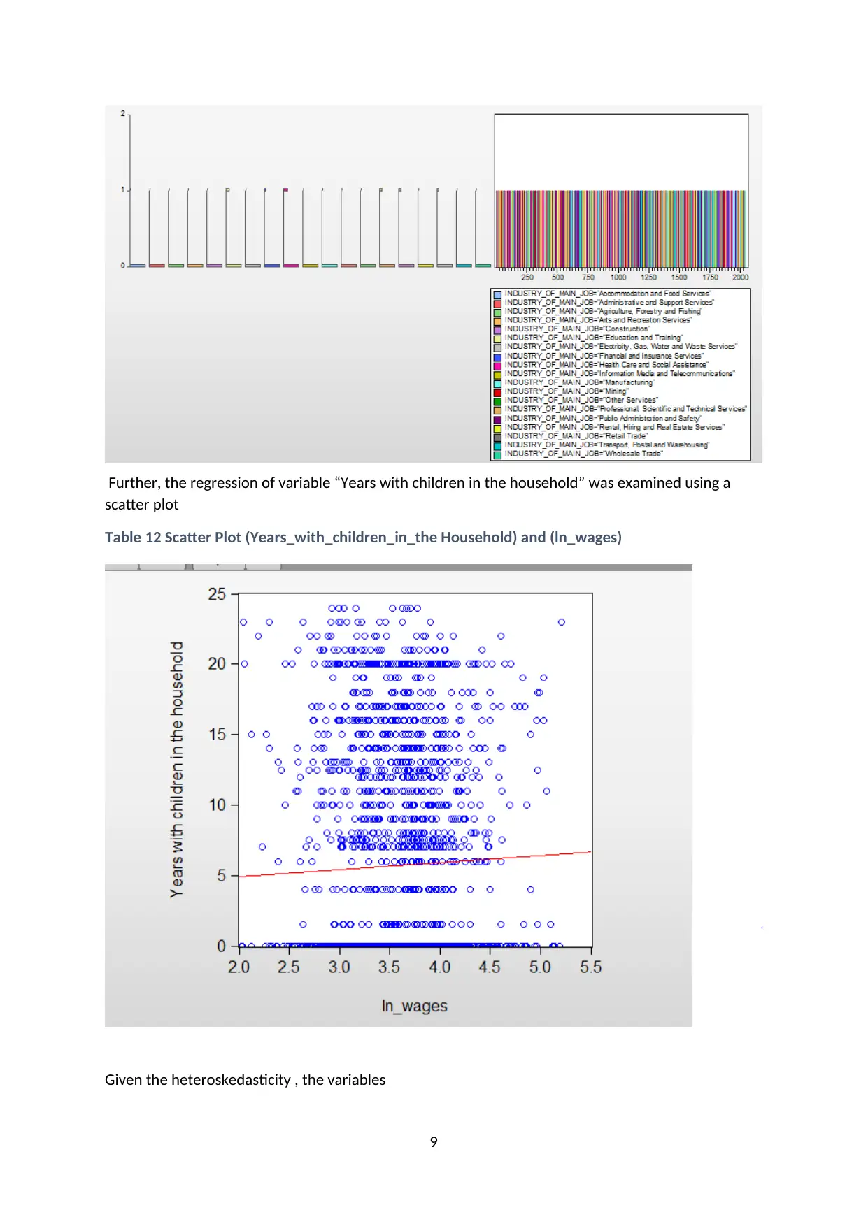
Further, the regression of variable “Years with children in the household” was examined using a
scatter plot
Table 12 Scatter Plot (Years_with_children_in_the Household) and (ln_wages)
Given the heteroskedasticity , the variables
9
scatter plot
Table 12 Scatter Plot (Years_with_children_in_the Household) and (ln_wages)
Given the heteroskedasticity , the variables
9
⊘ This is a preview!⊘
Do you want full access?
Subscribe today to unlock all pages.
Trusted by 1+ million students worldwide
1 out of 19
Related Documents


Your All-in-One AI-Powered Toolkit for Academic Success.
+13062052269
info@desklib.com
Available 24*7 on WhatsApp / Email
![[object Object]](/_next/static/media/star-bottom.7253800d.svg)
Unlock your academic potential
Copyright © 2020–2026 A2Z Services. All Rights Reserved. Developed and managed by ZUCOL.