Business Analytics Report: Gender Wage Gap at <University Name>
VerifiedAdded on 2022/09/18
|12
|2824
|20
Report
AI Summary
This business analytics report investigates the gender wage gap using a dataset of wages among men and women. The analysis employs descriptive statistics (mean, frequencies, percentages) and inferential statistics, including t-tests and correlations, to test the hypothesis that the gender wage gap is not statistically different from zero. The report includes data visualizations (scatter plots, histograms, line graphs, pie charts) created using Microsoft Excel. The literature review explores the significance of data in decision-making, particularly in policymaking, emphasizing the increasing participation of women in the labor market and factors influencing wage differences. The findings reveal differences in wages, age, and educational attainment between genders. The report concludes that there is no statistically significant difference between women's and men's wages and educational attainment. The study also analyses skewed distribution of the data.
Running head: BUSINESS ANALYTICS 1
Business analytics
<Name>
<University Name>
Business analytics
<Name>
<University Name>
Paraphrase This Document
Need a fresh take? Get an instant paraphrase of this document with our AI Paraphraser
BUSINESS ANALYTICS 2
Abstract
Generally, men participate more than women in labour force. Due to this, the dataset
utilized is quantitative in nature thus analyzed by use descriptive (mean, frequencies,
percentages) and inferential statistics. Statistical test including variances, skewed distribution,
standard deviations, paired-t-tests, spearman correlation were also used to test the hypothesized
statements. The Microsoft Office suite excel was used for drawing the visualizations. All tests of
significance were computed at α = 0.05. The hypothesis is that the gender wage gap is not
statistically different from zero hence make it more difficult to impose “equal pay” legislation.
Keywords: wage, gender, scatterplots, histogram, line graphs,
BUSINESS ANALYTICS 3
Table of Contents
Abstract............................................................................................................................................2
Introduction......................................................................................................................................2
Literature Review............................................................................................................................2
Data description...............................................................................................................................3
Descriptive and inferential statistics................................................................................................3
Skewed analysis...............................................................................................................................9
Summary of the findings...............................................................................................................10
Conclusion.....................................................................................................................................10
References......................................................................................................................................11
⊘ This is a preview!⊘
Do you want full access?
Subscribe today to unlock all pages.
Trusted by 1+ million students worldwide
BUSINESS ANALYTICS 4
Business analytics
Introduction
Basically, to present different data visualizations, excel Microsoft office suite has been
used to draw five different data visualizations (scatter plots, histograms, line graphs, Skewed
distribution, and pie charts) based on the chosen dataset. This dataset is about wages among men
and women.
The data has been prepared, explored, analyze, represented and validated on issues
relating to information technology, (Tan, 2018). Statistical test including skewed distribution was
also used to test the hypothesized statements, (Wilcox, & Rousselet, 2018). All tests of
significance were computed at α = 0.05, (Greenland, et al, 2016).
The information of the respondents such as Gender, Wage, Age, Educational attainment
in years, living in the City and the wage Level has been presented first by use of descriptive
statistics. After the descriptive statistics of the data have been discussed, the inferential statistics
have been presented based on the hypothesized statement which state that the gender wage gap is
not statistically different from zero hence make it more difficult to impose “equal pay”
legislation, (Hayes, 2017). In order to find the results of the hypothesis, data was first organized
by codding, cleaning and general data explorations, then data visualization and descriptive
findings were conducted, (Bernard, Wutich, and Ryan, 2016). Finally, the application and
problem-solving skills were utilized. Microsoft suite Excel was used to analyze the data, (Terry,
et, al, 2018).
Literature Review
Data is very important in decision making, especially in policymaking, (Dror, 2017). For
instance, before deciding on a policy like imposing pay legislation, the government and other
agencies should have the relevant evidence which is obtained from the right sources. Reading
and interpreting statistical information should be the basis of a decision-making process,
(Mertler, and Reinhart, 2016). For example, determining the age categories of the populations is
important because it will show the active population who are still fit for the employment
opportunities, thus helping in making effective decisions, (Granovetter, 2018).
Globally, the participation of people in any given labour market is dominated by men
more than women, (Basu, 2018). Recently, there has been an increase in female participation in
the labour market which is kind of sustained and substantial. Similarly, (Kirton, 2017),
established that females tend to participate more in the labour market than men. Therefore, there
is a need to establish gender participation difference in the labour market.
Furthermore, identifying the participation of women in the labour market is key since it is
a determinant by the government to come up with policies that address issues of the welfare
system, (Hakim, 2016). For instance, through the knowledge on gender participation in the
labour market, the government of any country can in one way or the other come up with policies
that encourage women to actively participate in the labour market as well as men, (Powell,
2018).
Additionally, there are several factors that can influence the participation of women in the
labour market. According, (Mihăilă, 2016), the availability of wage difference among men and
women can affect their participation in the labour market. The author confirmed that imposing
equal pay legislation in any government system will make a statistically significant difference
among gender when it comes to participation in any given labour market. In addition, age and
level of education influence the wage level of both men and women. In fact, the authors
confirmed that women tend to have high wage levels compared to men in a country where the
Paraphrase This Document
Need a fresh take? Get an instant paraphrase of this document with our AI Paraphraser
BUSINESS ANALYTICS 5
government imposed equal pay legislation.
Descriptive and inferential statistics
There are 500 observations for both men and women enclosed with six variables.
According to the results in Table, the mean wage for men; 7.24 bigger than that of women whose
mean wage is 3.58. The median wage value for men and women is 6.71 and 2.99 respectively. In
addition, the minimum and maximum values for wage value among women are constant at 25
while for men, the minimum wage value and maximum wage value is 26.58 and 26.07
respectively.
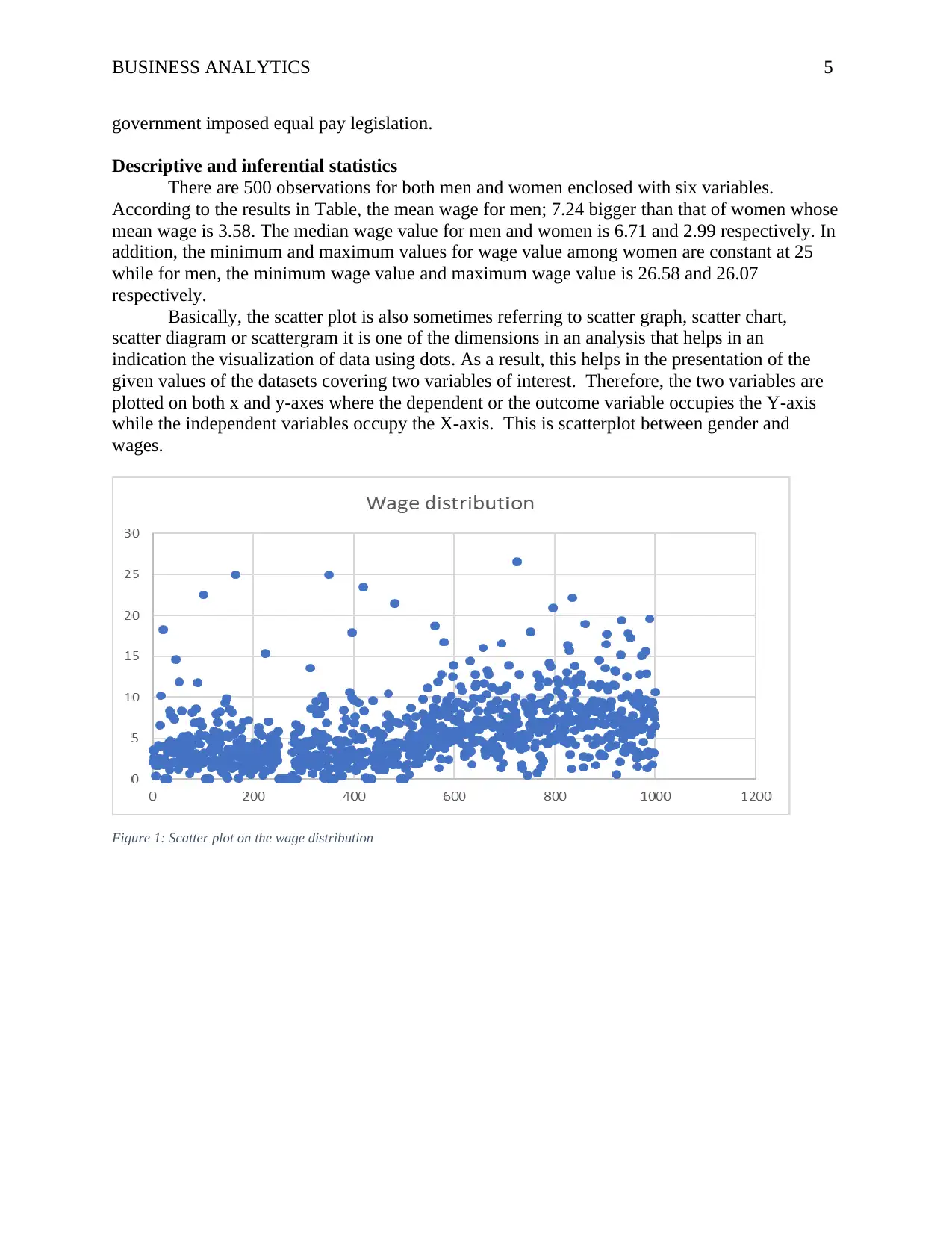
Basically, the scatter plot is also sometimes referring to scatter graph, scatter chart,
scatter diagram or scattergram it is one of the dimensions in an analysis that helps in an
indication the visualization of data using dots. As a result, this helps in the presentation of the
given values of the datasets covering two variables of interest. Therefore, the two variables are
plotted on both x and y-axes where the dependent or the outcome variable occupies the Y-axis
while the independent variables occupy the X-axis. This is scatterplot between gender and
wages.
Figure 1: Scatter plot on the wage distribution
government imposed equal pay legislation.
Descriptive and inferential statistics
There are 500 observations for both men and women enclosed with six variables.
According to the results in Table, the mean wage for men; 7.24 bigger than that of women whose
mean wage is 3.58. The median wage value for men and women is 6.71 and 2.99 respectively. In
addition, the minimum and maximum values for wage value among women are constant at 25
while for men, the minimum wage value and maximum wage value is 26.58 and 26.07
respectively.
Basically, the scatter plot is also sometimes referring to scatter graph, scatter chart,
scatter diagram or scattergram it is one of the dimensions in an analysis that helps in an
indication the visualization of data using dots. As a result, this helps in the presentation of the
given values of the datasets covering two variables of interest. Therefore, the two variables are
plotted on both x and y-axes where the dependent or the outcome variable occupies the Y-axis
while the independent variables occupy the X-axis. This is scatterplot between gender and
wages.
Figure 1: Scatter plot on the wage distribution
BUSINESS ANALYTICS 6
Table 1: Summary statistics on the wage and gender variables
Wage ($) Women Men
Mean 3.58 7.24
Median 2.99 6.71
Standard Deviation 3.39 3.60
First Quartile 1.64 4.83
Third Quartile 4.61 8.86
Interquartile Range 2.97 4.04
Minimum 0.00 0.51
Maximum 25.00 26.58
Range 25.00 26.07
Coefficient of Variation 0.95 0.50
Observations 500.00 500.00
The results in Table 2 show that majority of the women wage; 479 (95.2%) is between 0-
9 hours while for men wages, it is 378 (75.6%) as shown in Table 3. Furthermore, the women
and men wage between 10 to 14 accounted for 15 (3.00%) and 99 (19.80%) respectively as
shown in Table 2 and 3. Finally, the women and men wages for 15 and more is 9 (1.80%) and 23
(4.60%) respectively as shown in Table 2 and 3. The mean women and men wage are 3.58; the
standard deviation of 3.39 and 7.24; the standard deviation of 3.60 respectively.
Table 2: Women wage
Freq. %
0 to 9 476 95.20%
10 to 14 15 3.00%
15+ 9 1.80%
Total 500 100.00%
Mean 3.58
Standard Deviation 3.39
Range 25
Table 3: Men wage
Freq. %
0 to 9 378 75.60%
10 to 14 99 19.80%
15+ 23 4.60%
Total 500 100.00%
Mean 7.24
Standard Deviation 3.60
Range 26.0652
In order to establish whether there is a statistically significant difference between the
women and men wages, a paired t-test was conducted between the women and men wages.
⊘ This is a preview!⊘
Do you want full access?
Subscribe today to unlock all pages.
Trusted by 1+ million students worldwide
BUSINESS ANALYTICS 7
According to the findings in Table 4, there is no statistically significant association between
women and men wages since the p-value is >0.05.
Table 4: Comparison of women and men wages
t-Test: Paired Two Sample for Means
Variable 1 Variable 2
Mean 3.576095 7.238361
Variance 11.5325 13.02158
Observations 500 500
Pearson Correlation 0.174665
Hypothesized Mean Difference 0
Df 499
t Stat -18.1875
P(T<=t) one-tail 2.21E-57
t Critical one-tail 1.647913
P(T<=t) two-tail 4.42E-57
t Critical two-tail 1.964729
Table 5: Age Category in Years
Women Men
Age in years Freq. % Freq. %
0-30 25 5.00% 10 2.00%
31-40 202 40.40% 157 31.40%
41-50 190 38.00% 203 40.60%
51+ 83 16.60% 130 26.00%
Total 500 100.00% 500 100.00%
Mean 41.984 44.662
Standard Deviation 7.8133056 8.0039838
Range 30 30
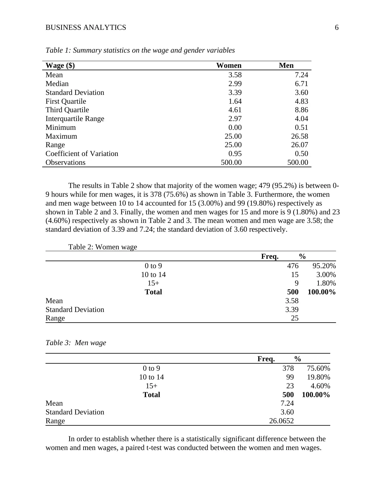
According to the results in Table 5, majority of women; 202 (40.4%) were between 31-40
years old while the majority of the men; 203 (40.60%) were aged from 41-50 years. In addition,
190 (38.0%) of women were 41-50 years old while 157 (31.40%) of the men were 31-40 years
old. The older women and men; 51+ years accounted for 83 (16.60%) and 130 (26.00%)
respectively. In a nutshell, the husband seems to be older in years as compared to wives. The
mean age in years for wives is 41.98 with a standard deviation of 7.81 lower than that of
husbands at 44.66 and a standard deviation of 8 respectively. The same results on age category
have been summarized in Figure 1 below.
According to the findings in Table 4, there is no statistically significant association between
women and men wages since the p-value is >0.05.
Table 4: Comparison of women and men wages
t-Test: Paired Two Sample for Means
Variable 1 Variable 2
Mean 3.576095 7.238361
Variance 11.5325 13.02158
Observations 500 500
Pearson Correlation 0.174665
Hypothesized Mean Difference 0
Df 499
t Stat -18.1875
P(T<=t) one-tail 2.21E-57
t Critical one-tail 1.647913
P(T<=t) two-tail 4.42E-57
t Critical two-tail 1.964729
Table 5: Age Category in Years
Women Men
Age in years Freq. % Freq. %
0-30 25 5.00% 10 2.00%
31-40 202 40.40% 157 31.40%
41-50 190 38.00% 203 40.60%
51+ 83 16.60% 130 26.00%
Total 500 100.00% 500 100.00%
Mean 41.984 44.662
Standard Deviation 7.8133056 8.0039838
Range 30 30
According to the results in Table 5, majority of women; 202 (40.4%) were between 31-40
years old while the majority of the men; 203 (40.60%) were aged from 41-50 years. In addition,
190 (38.0%) of women were 41-50 years old while 157 (31.40%) of the men were 31-40 years
old. The older women and men; 51+ years accounted for 83 (16.60%) and 130 (26.00%)
respectively. In a nutshell, the husband seems to be older in years as compared to wives. The
mean age in years for wives is 41.98 with a standard deviation of 7.81 lower than that of
husbands at 44.66 and a standard deviation of 8 respectively. The same results on age category
have been summarized in Figure 1 below.
Paraphrase This Document
Need a fresh take? Get an instant paraphrase of this document with our AI Paraphraser
BUSINESS ANALYTICS 8
Figure 2: Histogram- Age Distribution among gender
In order to establish whether there is a statistically significant difference between the
means of age in years, a paired t-test was conducted between the women and women’s age in
years. According to the findings in Table 6, there is no statistically significant association
between women's and men’s age in years since the p-value is >0.05.
Table 6: Comparisons of age in years
t-Test: Paired Two Sample for Means
Variable 1 Variable 2
Mean 41.984 44.662
Variance 61.17008 64.19214
Observations 500 500
Pearson Correlation 0.899821
Hypothesized Mean Difference 0
Df 499
t Stat -16.8755
P(T<=t) one-tail 3.5E-51
t Critical one-tail 1.647913
P(T<=t) two-tail 7E-51
t Critical two-tail 1.964729
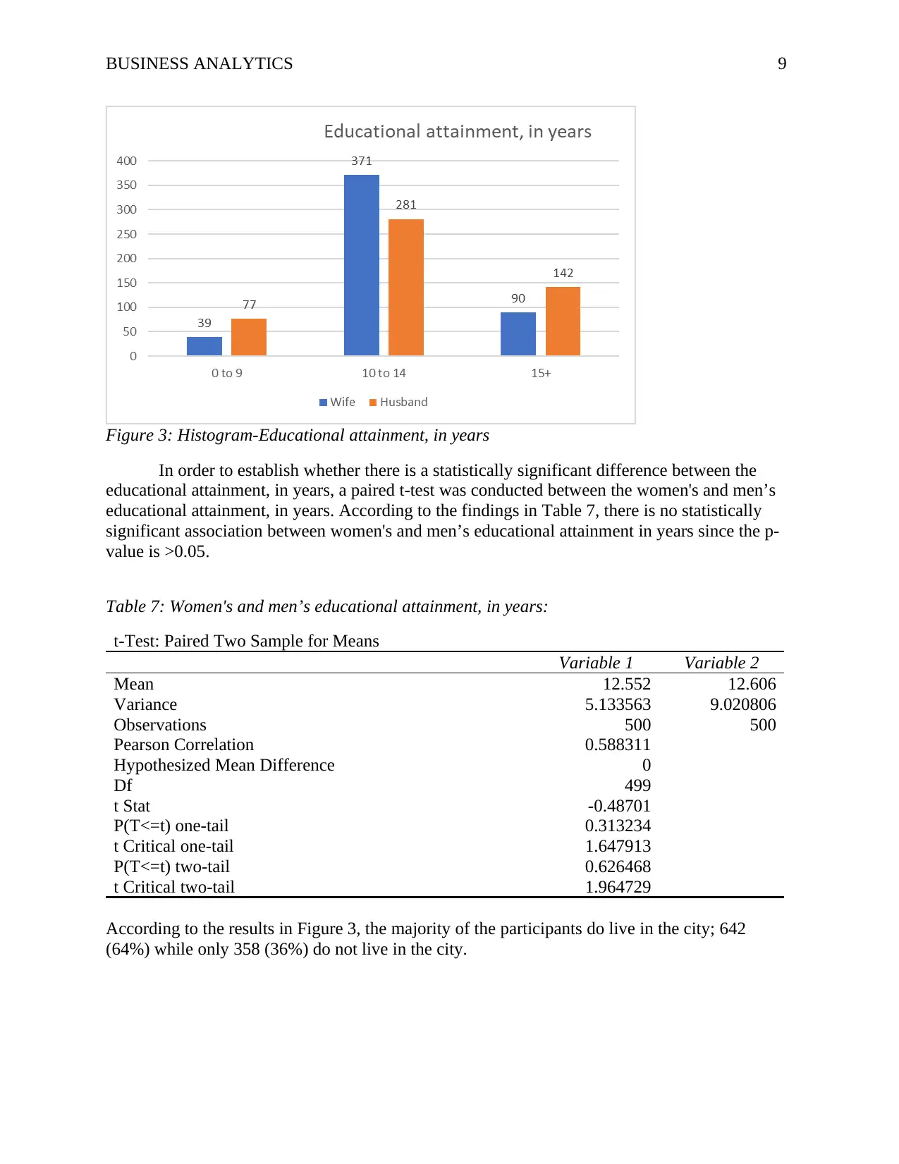
According to the results in Figure 2, majority of the women; 371 had the highest
educational attachment in years of 10 to 14 while men were only 281 for the same educational
attachment in years of 10 to 14. The mean educational attachment in years for women is 12.55
with a standard deviation of 2.26 while for men, the mean is 12.61 and a standard deviation of
3.00 which are all higher than that of women.
Figure 2: Histogram- Age Distribution among gender
In order to establish whether there is a statistically significant difference between the
means of age in years, a paired t-test was conducted between the women and women’s age in
years. According to the findings in Table 6, there is no statistically significant association
between women's and men’s age in years since the p-value is >0.05.
Table 6: Comparisons of age in years
t-Test: Paired Two Sample for Means
Variable 1 Variable 2
Mean 41.984 44.662
Variance 61.17008 64.19214
Observations 500 500
Pearson Correlation 0.899821
Hypothesized Mean Difference 0
Df 499
t Stat -16.8755
P(T<=t) one-tail 3.5E-51
t Critical one-tail 1.647913
P(T<=t) two-tail 7E-51
t Critical two-tail 1.964729
According to the results in Figure 2, majority of the women; 371 had the highest
educational attachment in years of 10 to 14 while men were only 281 for the same educational
attachment in years of 10 to 14. The mean educational attachment in years for women is 12.55
with a standard deviation of 2.26 while for men, the mean is 12.61 and a standard deviation of
3.00 which are all higher than that of women.
BUSINESS ANALYTICS 9
Figure 3: Histogram-Educational attainment, in years
In order to establish whether there is a statistically significant difference between the
educational attainment, in years, a paired t-test was conducted between the women's and men’s
educational attainment, in years. According to the findings in Table 7, there is no statistically
significant association between women's and men’s educational attainment in years since the p-
value is >0.05.
Table 7: Women's and men’s educational attainment, in years:
t-Test: Paired Two Sample for Means
Variable 1 Variable 2
Mean 12.552 12.606
Variance 5.133563 9.020806
Observations 500 500
Pearson Correlation 0.588311
Hypothesized Mean Difference 0
Df 499
t Stat -0.48701
P(T<=t) one-tail 0.313234
t Critical one-tail 1.647913
P(T<=t) two-tail 0.626468
t Critical two-tail 1.964729
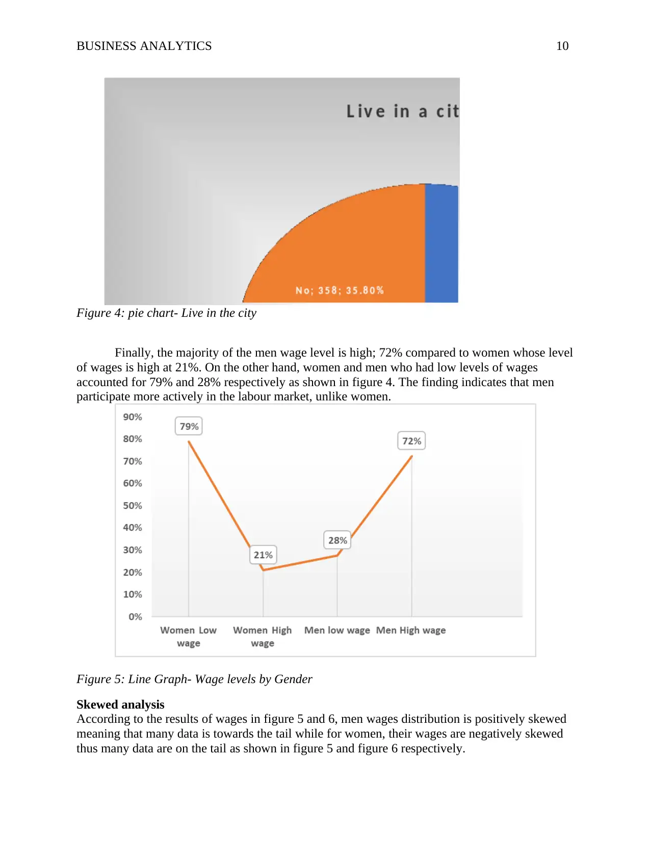
According to the results in Figure 3, the majority of the participants do live in the city; 642
(64%) while only 358 (36%) do not live in the city.
Figure 3: Histogram-Educational attainment, in years
In order to establish whether there is a statistically significant difference between the
educational attainment, in years, a paired t-test was conducted between the women's and men’s
educational attainment, in years. According to the findings in Table 7, there is no statistically
significant association between women's and men’s educational attainment in years since the p-
value is >0.05.
Table 7: Women's and men’s educational attainment, in years:
t-Test: Paired Two Sample for Means
Variable 1 Variable 2
Mean 12.552 12.606
Variance 5.133563 9.020806
Observations 500 500
Pearson Correlation 0.588311
Hypothesized Mean Difference 0
Df 499
t Stat -0.48701
P(T<=t) one-tail 0.313234
t Critical one-tail 1.647913
P(T<=t) two-tail 0.626468
t Critical two-tail 1.964729
According to the results in Figure 3, the majority of the participants do live in the city; 642
(64%) while only 358 (36%) do not live in the city.
⊘ This is a preview!⊘
Do you want full access?
Subscribe today to unlock all pages.
Trusted by 1+ million students worldwide
BUSINESS ANALYTICS 10
Figure 4: pie chart- Live in the city
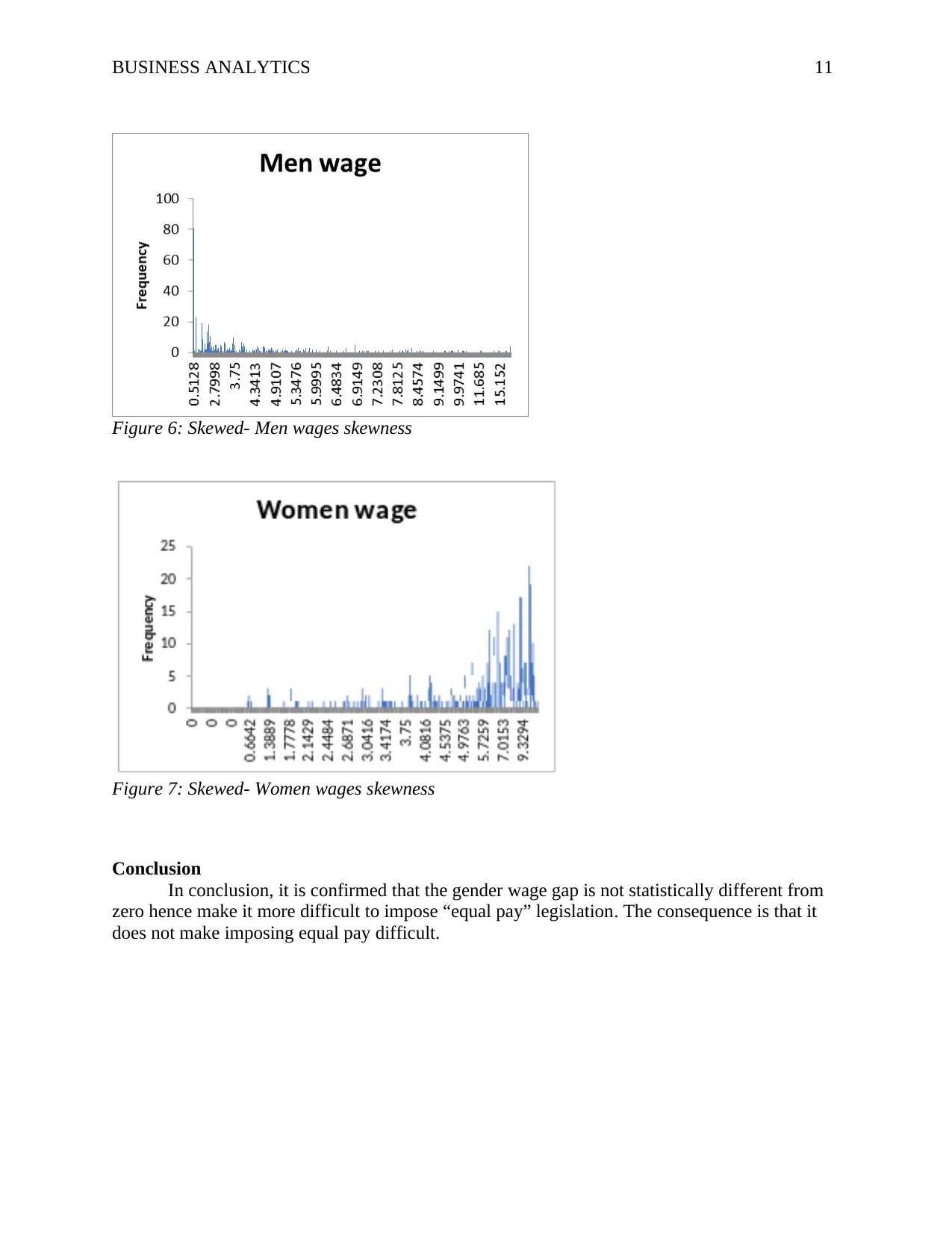
Finally, the majority of the men wage level is high; 72% compared to women whose level
of wages is high at 21%. On the other hand, women and men who had low levels of wages
accounted for 79% and 28% respectively as shown in figure 4. The finding indicates that men
participate more actively in the labour market, unlike women.
Figure 5: Line Graph- Wage levels by Gender
Skewed analysis
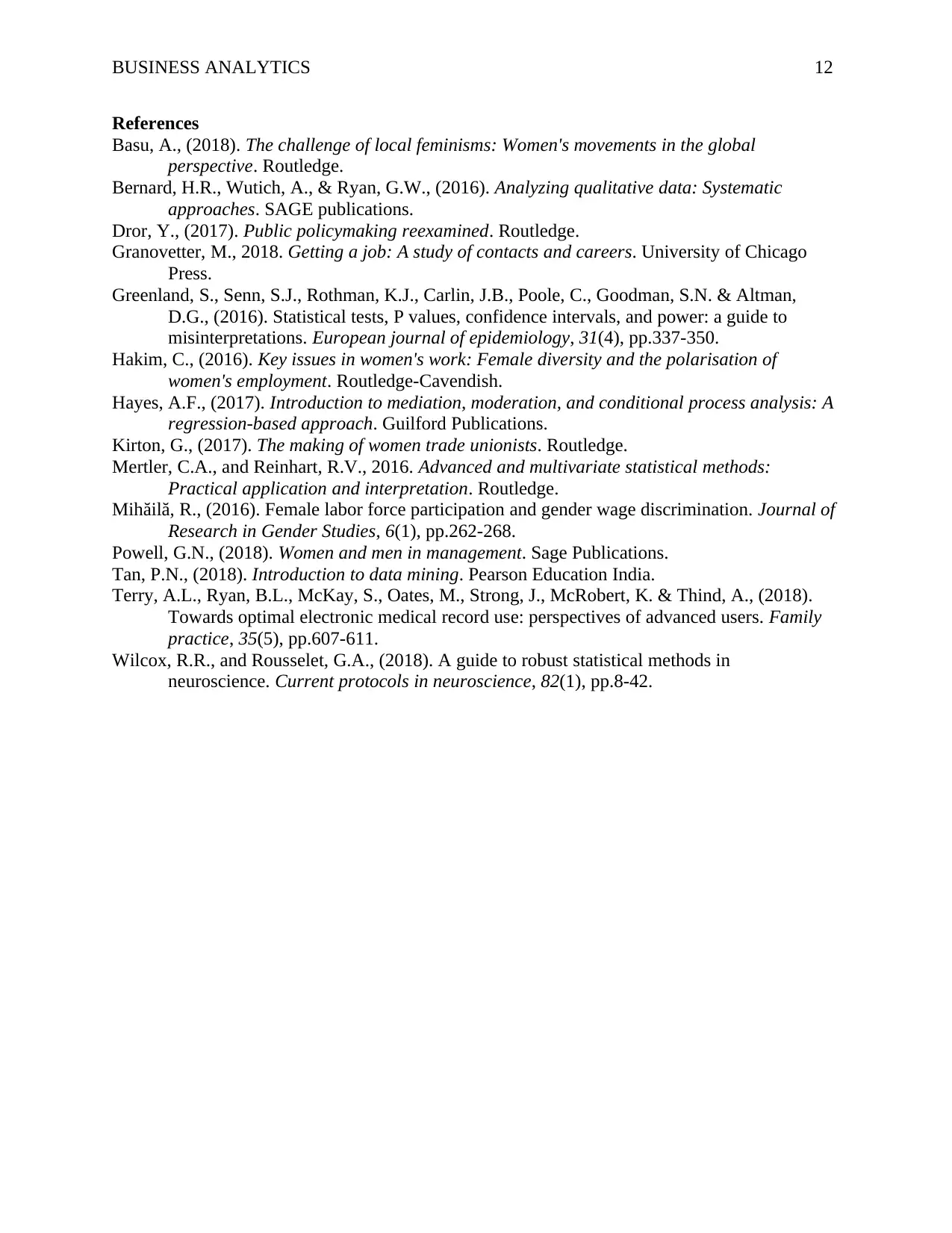
According to the results of wages in figure 5 and 6, men wages distribution is positively skewed
meaning that many data is towards the tail while for women, their wages are negatively skewed
thus many data are on the tail as shown in figure 5 and figure 6 respectively.
Figure 4: pie chart- Live in the city
Finally, the majority of the men wage level is high; 72% compared to women whose level
of wages is high at 21%. On the other hand, women and men who had low levels of wages
accounted for 79% and 28% respectively as shown in figure 4. The finding indicates that men
participate more actively in the labour market, unlike women.
Figure 5: Line Graph- Wage levels by Gender
Skewed analysis
According to the results of wages in figure 5 and 6, men wages distribution is positively skewed
meaning that many data is towards the tail while for women, their wages are negatively skewed
thus many data are on the tail as shown in figure 5 and figure 6 respectively.
Paraphrase This Document
Need a fresh take? Get an instant paraphrase of this document with our AI Paraphraser
BUSINESS ANALYTICS 11
Figure 6: Skewed- Men wages skewness
Figure 7: Skewed- Women wages skewness
Conclusion
In conclusion, it is confirmed that the gender wage gap is not statistically different from
zero hence make it more difficult to impose “equal pay” legislation. The consequence is that it
does not make imposing equal pay difficult.
BUSINESS ANALYTICS 12
References
Basu, A., (2018). The challenge of local feminisms: Women's movements in the global
perspective. Routledge.
Bernard, H.R., Wutich, A., & Ryan, G.W., (2016). Analyzing qualitative data: Systematic
approaches. SAGE publications.
Dror, Y., (2017). Public policymaking reexamined. Routledge.
Granovetter, M., 2018. Getting a job: A study of contacts and careers. University of Chicago
Press.
Greenland, S., Senn, S.J., Rothman, K.J., Carlin, J.B., Poole, C., Goodman, S.N. & Altman,
D.G., (2016). Statistical tests, P values, confidence intervals, and power: a guide to
misinterpretations. European journal of epidemiology, 31(4), pp.337-350.
Hakim, C., (2016). Key issues in women's work: Female diversity and the polarisation of
women's employment. Routledge-Cavendish.
Hayes, A.F., (2017). Introduction to mediation, moderation, and conditional process analysis: A
regression-based approach. Guilford Publications.
Kirton, G., (2017). The making of women trade unionists. Routledge.
Mertler, C.A., and Reinhart, R.V., 2016. Advanced and multivariate statistical methods:
Practical application and interpretation. Routledge.
Mihăilă, R., (2016). Female labor force participation and gender wage discrimination. Journal of
Research in Gender Studies, 6(1), pp.262-268.
Powell, G.N., (2018). Women and men in management. Sage Publications.
Tan, P.N., (2018). Introduction to data mining. Pearson Education India.
Terry, A.L., Ryan, B.L., McKay, S., Oates, M., Strong, J., McRobert, K. & Thind, A., (2018).
Towards optimal electronic medical record use: perspectives of advanced users. Family
practice, 35(5), pp.607-611.
Wilcox, R.R., and Rousselet, G.A., (2018). A guide to robust statistical methods in
neuroscience. Current protocols in neuroscience, 82(1), pp.8-42.
⊘ This is a preview!⊘
Do you want full access?
Subscribe today to unlock all pages.
Trusted by 1+ million students worldwide
1 out of 12

Your All-in-One AI-Powered Toolkit for Academic Success.
+13062052269
info@desklib.com
Available 24*7 on WhatsApp / Email
![[object Object]](/_next/static/media/star-bottom.7253800d.svg)
Unlock your academic potential
Copyright © 2020–2026 A2Z Services. All Rights Reserved. Developed and managed by ZUCOL.