Research Report: Analyzing GFCF and GDP in the Australian Economy

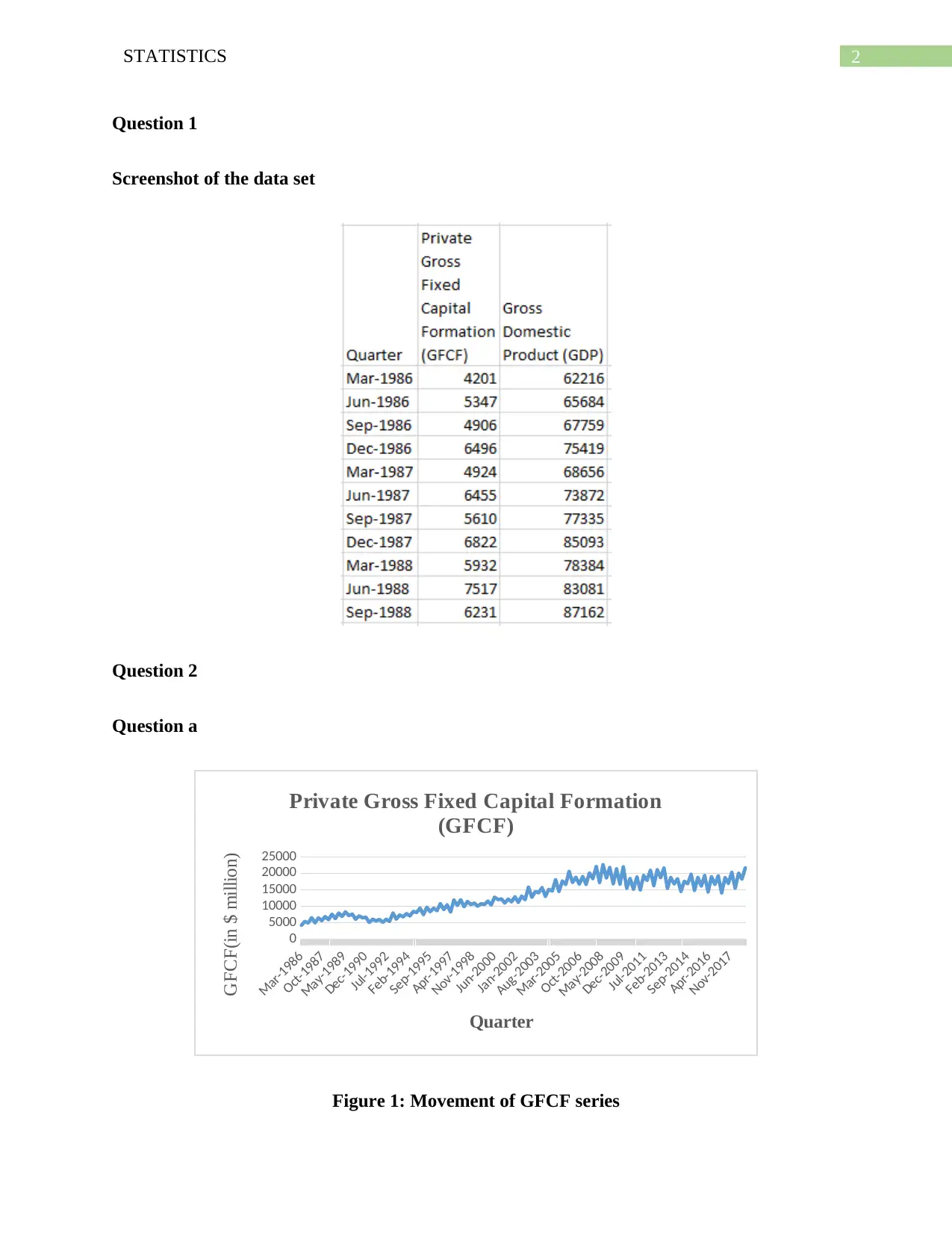
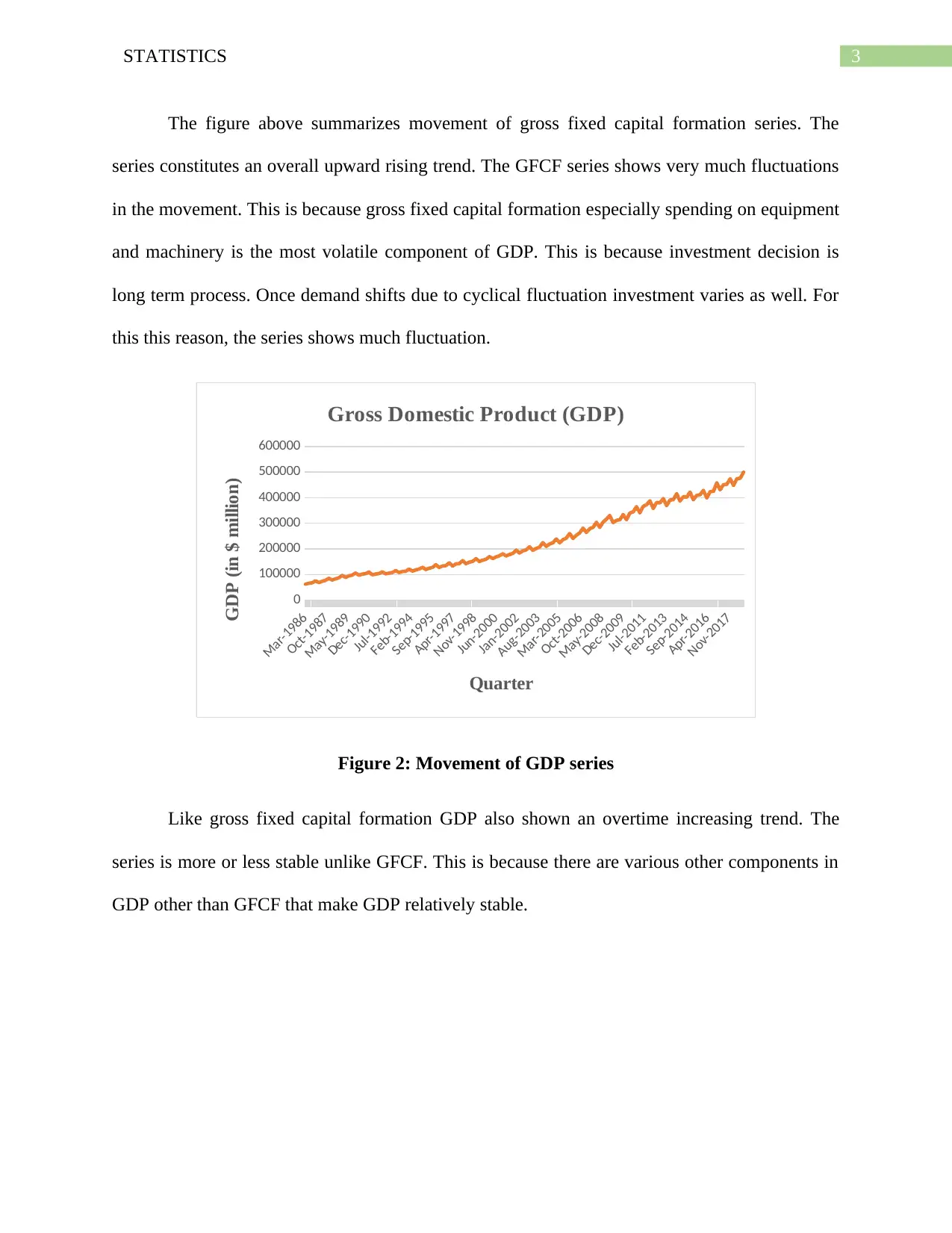
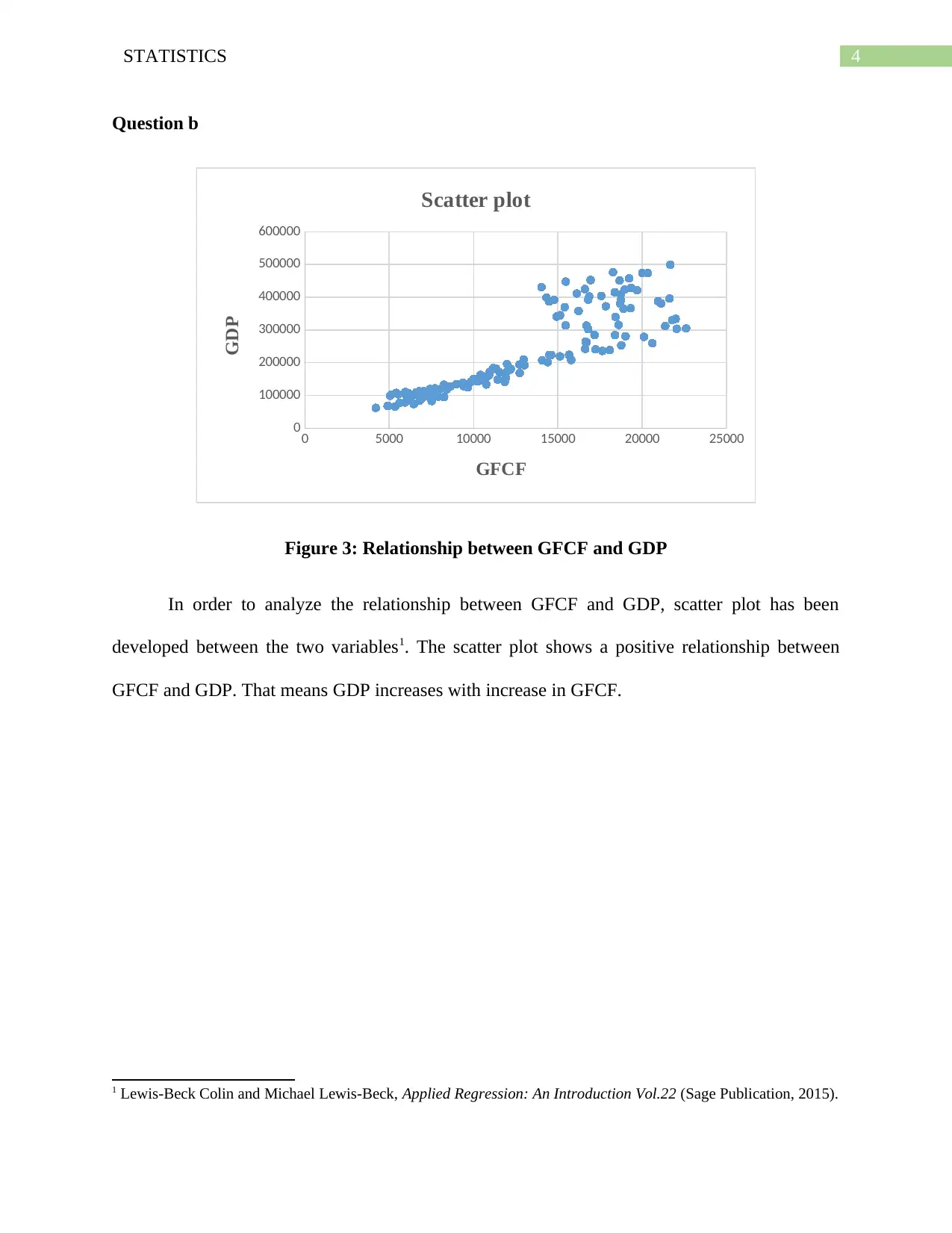
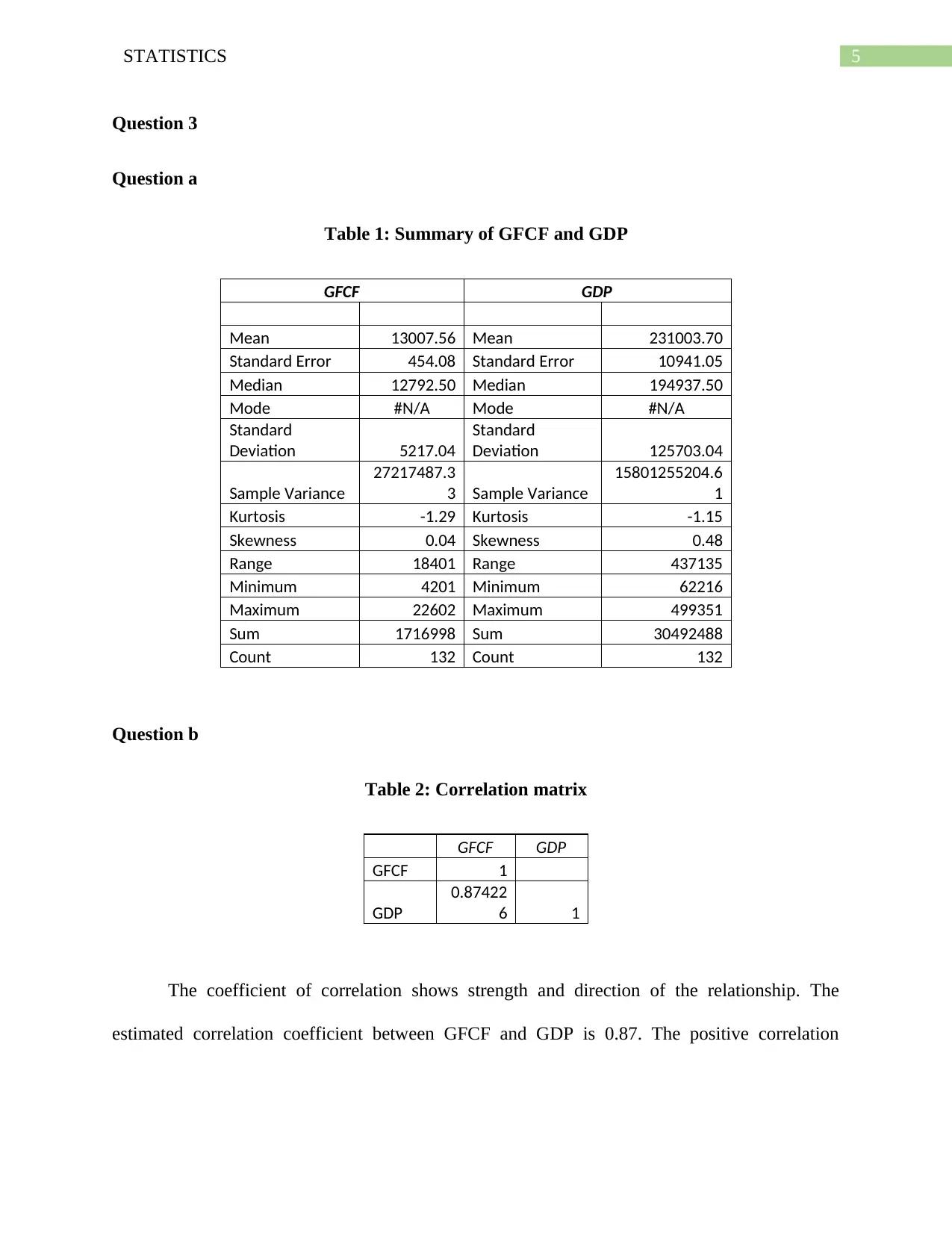
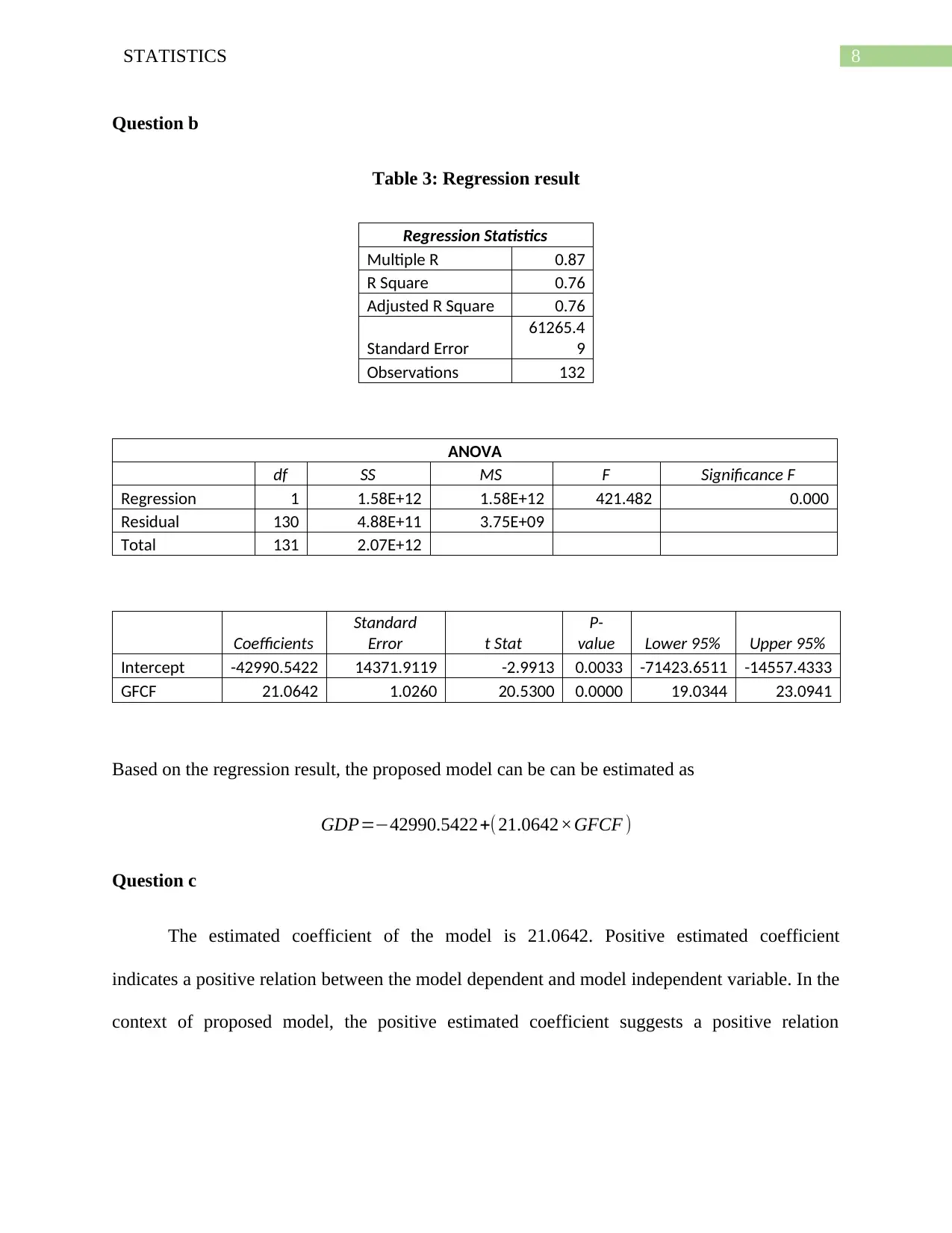
This report examines the relationship between Private Gross Fixed Capital Formation (GFCF) and Gross Domestic Product (GDP) in Australia, utilizing quarterly data from March 1986 to December 2018. The analysis includes trend analysis, correlation, and regression analysis to determine if GFCF is a good predictor of GDP. The report presents descriptive statistics, scatter plots, and regression results, including coefficients, standard errors, and p-values. Hypothesis testing is conducted to assess the significance of the linear relationship between GFCF and GDP. The findings indicate a positive and statistically significant relationship, with the model showing a good fit, explaining a substantial portion of the variation in GDP. The conclusion supports the claim that GFCF is a significant predictor of GDP, highlighting the importance of investment in machinery and equipment for economic growth. The report also includes a summary of the findings and references used.

Running head: STATISTICS
Statistics
Name of the Student
Name of the University
Course ID

1STATISTICS
Table of Contents
Question 1........................................................................................................................................2
Question 2........................................................................................................................................2
Question a....................................................................................................................................2
Question b....................................................................................................................................4
Question 3........................................................................................................................................5
Question a....................................................................................................................................5
Question b....................................................................................................................................5
Question 4........................................................................................................................................6
Question a....................................................................................................................................6
Question b....................................................................................................................................7
Question c....................................................................................................................................7
Question 5........................................................................................................................................8
Question a....................................................................................................................................8
Question b..................................................................................................................................10
Question 6......................................................................................................................................10
Summary report.........................................................................................................................10
References......................................................................................................................................12

2STATISTICS
Question 1
Screenshot of the data set
Question 2
Question a
Mar-1986
Oct-1987
May-1989
Dec-1990
Jul-1992
Feb-1994
Sep-1995
Apr-1997
Nov-1998
Jun-2000
Jan-2002
Aug-2003
Mar-2005
Oct-2006
May-2008
Dec-2009
Jul-2011
Feb-2013
Sep-2014
Apr-2016
Nov-2017
0
5000
10000
15000
20000
25000
Private Gross Fixed Capital Formation
(GFCF)
Quarter
GFCF(in $ million)
Figure 1: Movement of GFCF series

3STATISTICS
The figure above summarizes movement of gross fixed capital formation series. The
series constitutes an overall upward rising trend. The GFCF series shows very much fluctuations
in the movement. This is because gross fixed capital formation especially spending on equipment
and machinery is the most volatile component of GDP. This is because investment decision is
long term process. Once demand shifts due to cyclical fluctuation investment varies as well. For
this this reason, the series shows much fluctuation.
Mar-1986
Oct-1987
May-1989
Dec-1990
Jul-1992
Feb-1994
Sep-1995
Apr-1997
Nov-1998
Jun-2000
Jan-2002
Aug-2003
Mar-2005
Oct-2006
May-2008
Dec-2009
Jul-2011
Feb-2013
Sep-2014
Apr-2016
Nov-2017
0
100000
200000
300000
400000
500000
600000
Gross Domestic Product (GDP)
Quarter
GDP (in $ million)
Figure 2: Movement of GDP series
Like gross fixed capital formation GDP also shown an overtime increasing trend. The
series is more or less stable unlike GFCF. This is because there are various other components in
GDP other than GFCF that make GDP relatively stable.

4STATISTICS
Question b
0 5000 10000 15000 20000 25000
0
100000
200000
300000
400000
500000
600000
Scatter plot
GFCF
GDP
Figure 3: Relationship between GFCF and GDP
In order to analyze the relationship between GFCF and GDP, scatter plot has been
developed between the two variables1. The scatter plot shows a positive relationship between
GFCF and GDP. That means GDP increases with increase in GFCF.
1 Lewis-Beck Colin and Michael Lewis-Beck, Applied Regression: An Introduction Vol.22 (Sage Publication, 2015).

5STATISTICS
Question 3
Question a
Table 1: Summary of GFCF and GDP
GFCF GDP
Mean 13007.56 Mean 231003.70
Standard Error 454.08 Standard Error 10941.05
Median 12792.50 Median 194937.50
Mode #N/A Mode #N/A
Standard
Deviation 5217.04
Standard
Deviation 125703.04
Sample Variance
27217487.3
3 Sample Variance
15801255204.6
1
Kurtosis -1.29 Kurtosis -1.15
Skewness 0.04 Skewness 0.48
Range 18401 Range 437135
Minimum 4201 Minimum 62216
Maximum 22602 Maximum 499351
Sum 1716998 Sum 30492488
Count 132 Count 132
Question b
Table 2: Correlation matrix
GFCF GDP
GFCF 1
GDP
0.87422
6 1
The coefficient of correlation shows strength and direction of the relationship. The
estimated correlation coefficient between GFCF and GDP is 0.87. The positive correlation

6STATISTICS
coefficient suggests a positive relation between GDP and GFCF2. In other words, increase in
GFCF increase GDP as well. The obtained value of correlation coefficient is closer towards 1,
the line of perfect correlation. This therefore indicates a strong relationship between the two
variables.
Question 4
Question a
In order to explain the relationship between GFCF and GDP following has been
developed
GDP=β0+(β1 × GFCF)
‘ β0’ is the intercept terms of the regression and ‘ β1’ is the slope coefficient. In the above model,
GDP is taken as dependent variable and GFCF is taken as independent variable. Gross domestic
product (GDP) is a measure expressing monetary value of goods and services produced within a
nation. GDP is often expressed as a sum of expenditure on four different components –
consumption, investment, government expenditure and net export. Changes on any one
component leads to a change in GDP. Now spending on machinery and equipment is a part of
gross fixed capital formation which is include as investment in GDP computation3. Therefore,
changes in spending on machinery and equipment affects GDP through changing investment.
Following the macroeconomic theory in the above model GDP is considered as dependent
variable and GFCF is considered as independent variable.
2 Asis Kumar Chattopadhyay and Tanuka Chattopadhyay, Statistical Methods For Astronomical Data
Analysis (Springer New York, 2014).
3 Sebastian Dullien et al, Macroeconomics In Context (Routledge, 2015).

7STATISTICS

8STATISTICS
Question b
Table 3: Regression result
Regression Statistics
Multiple R 0.87
R Square 0.76
Adjusted R Square 0.76
Standard Error
61265.4
9
Observations 132
ANOVA
df SS MS F Significance F
Regression 1 1.58E+12 1.58E+12 421.482 0.000
Residual 130 4.88E+11 3.75E+09
Total 131 2.07E+12
Coefficients
Standard
Error t Stat
P-
value Lower 95% Upper 95%
Intercept -42990.5422 14371.9119 -2.9913 0.0033 -71423.6511 -14557.4333
GFCF 21.0642 1.0260 20.5300 0.0000 19.0344 23.0941
Based on the regression result, the proposed model can be can be estimated as
GDP=−42990.5422+(21.0642×GFCF )
Question c
The estimated coefficient of the model is 21.0642. Positive estimated coefficient
indicates a positive relation between the model dependent and model independent variable. In the
context of proposed model, the positive estimated coefficient suggests a positive relation

9STATISTICS
between GFCF and GDP4. More preciously, GDP increases with an associated increase in GFCF
and decreases with decrease in GFCF.
Question 5
Question a
Test for significance of linear relationship between GFCF and GDP.
Hypotheses
Null Hypothesis (H0): The coefficient of GFCF is not significantly different from zero.
β1=0
Alternative Hypothesis (H1): The coefficient of GFCF is significantly different from zero.
β1 ≠ 0
Level of significance
The test has been conducted based on 5% level of significance. The value of chosen level
of significance thus is 0.05.
Level of significance ( α ) =0.05
Test statistics
In order to conduct the proposed hypothesis test ‘t’ test is to be conducted. The estimate
for t statistics is given as follows
4 Samprit Chatterjee and Ali S Hadi, Regression Analysis By Example (John Wiley & Sons, 2015).

10STATISTICS
T 0= ^β1− β1
SE ( β1)
This follows t distribution with (n – 2) degrees of freedom and α
2 level of significance.
Rejection region
The null hypothesis is rejected if computed T value fall outside the following region
−t α
2 ,n−2 <T0 <t α
2 ,n−2
−t α
2 ,n−2 and t α
2 ,n−2 are the critical t values for two sided hypothesis5. In other the null hypothesis
is rejected if
|T |>t α
2 ,n−2
Calculation
From the regression result the estimated value of the coefficient is 21.0642. The
associated standard error is 1.0260. Therefore, T value can be computed as
T 0=
^β1−β1
SE ( β1 ) 0.025 , 130
¿ 21.0642
1.0260
¿ 20.5300
Conclusion
5 Anthony R. Ives, "For Testing The Significance Of Regression Coefficients, Go Ahead And Log-Transform Count
Data" (2015) 6(7) Methods in Ecology and Evolution.

11STATISTICS
The critical t value for 130 degrees of freedom 0.025 significance level is 1.9784. As the
computed T is greater than critical t, the null hypothesis that the coefficient is not significantly
different zero has been accepted. This in turn means that there exists a valid statistical relation
between GDP and GFCF.
Question b
Goodness of fit of a model depends on the explanatory power of the model. In other
words, more variation in the dependent variable is explained by the independent variable better
fit is the model. This can be understood from the value of R square or coefficient of
determination6. The R square value of the model is 0.76. This indicates that the independent
variable (GFCF) account 76 percent variation in the dependent variable (GDP). As GFCF
explains most of the variation in GDP, the model can be said as a good fit model.
Question 6
Summary report
The report aims to analyze whether Private Gross Fixed Capital Formation is a good
predictor of Gross Domestic Product of the country. Gross Domestic Product of a nation
measures sum of values of all produced goods and services in the country7. Total gross fixed
capital formation presents changes in physical stock of capital in a nation and included in GDP
as investment expenditure. This includes expenditure carried out by both public and private.
Now private fixed capital formation include investment made by private individual on machinery
and equipment. An increase in investment in machinery and equipment likely to increase
6 John Fox, Applied Regression Analysis And Generalized Linear Models (SAGE Publications, 2015).
7 Ben J Heijdra, Foundations Of Modern Macroeconomics (Oxford university press, 2017).