MAE203: Detailed Analysis of the Global Economy Written Assignment
VerifiedAdded on 2022/05/31
|17
|3156
|84
Report
AI Summary
This report, prepared as an MAE203 assignment, delves into the intricacies of the global economy through detailed analysis and comparisons. The report examines the relationship between Total Factor Productivity (TFP) and real GDP across various countries, including Australia, China, France, Germany, Japan, Spain, the United Kingdom, and the USA, highlighting diverse growth patterns and economic trends. It also analyzes GDP per capita, import values, government debt, and government final expenditure for several nations, providing a comprehensive overview of economic performance and governmental influence. Furthermore, the report explores the correlation between unfilled job vacancies and the unemployment rate in Australia, discussing the implications of skill shortages and economic openness. The assignment concludes with a case study on Sheng Long Bio-Tech International Co.Ltd, where the author discusses the suitability of an economist role within the company, emphasizing data-driven decision-making and analytical skills.

1
MAE203 – THE GLOBAL ECONOMY
WRITTEN ASSIGNMENT
MAE203 – THE GLOBAL ECONOMY
WRITTEN ASSIGNMENT
Paraphrase This Document
Need a fresh take? Get an instant paraphrase of this document with our AI Paraphraser

2
Contents
Part 1..........................................................................................................................................3
Part B........................................................................................................................................11
Part C........................................................................................................................................12
Reference..................................................................................................................................14
3
Part 1
Question 1
Case of Australia
1960
1963
1966
1969
1972
1975
1978
1981
1984
1987
1990
1993
1996
1999
2002
2005
2008
2011
2014
2017
0.00
200000.00
400000.00
600000.00
800000.00
1000000.00
1200000.00
0.00
0.20
0.40
0.60
0.80
1.00
1.20
TFP and real GDP for australia
Real GDP Total factor productivity
Year
Real GDP
Total Factor Productivity
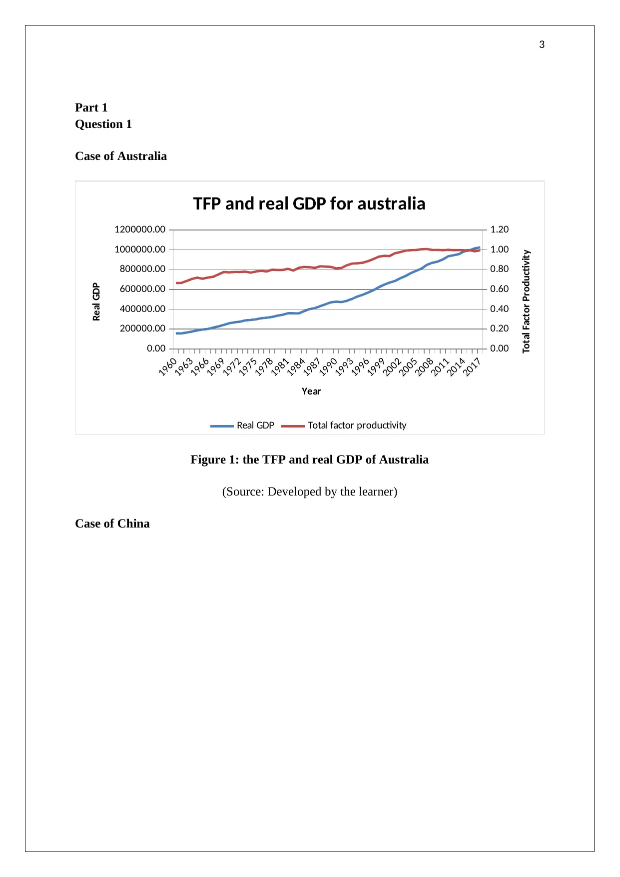
Figure 1: the TFP and real GDP of Australia
(Source: Developed by the learner)
Case of China
Part 1
Question 1
Case of Australia
1960
1963
1966
1969
1972
1975
1978
1981
1984
1987
1990
1993
1996
1999
2002
2005
2008
2011
2014
2017
0.00
200000.00
400000.00
600000.00
800000.00
1000000.00
1200000.00
0.00
0.20
0.40
0.60
0.80
1.00
1.20
TFP and real GDP for australia
Real GDP Total factor productivity
Year
Real GDP
Total Factor Productivity
Figure 1: the TFP and real GDP of Australia
(Source: Developed by the learner)
Case of China
⊘ This is a preview!⊘
Do you want full access?
Subscribe today to unlock all pages.
Trusted by 1+ million students worldwide
4
1952
1956
1960
1964
1968
1972
1976
1980
1984
1988
1992
1996
2000
2004
2008
2012
2016
0.00
0.20
0.40
0.60
0.80
1.00
1.20
0.00
2000000.00
4000000.00
6000000.00
8000000.00
10000000.00
12000000.00
14000000.00
16000000.00
18000000.00
20000000.00
TFP and real GDP of China
Total factor productivity Real GDP
Year
Real GDP
Total Factor Productivity
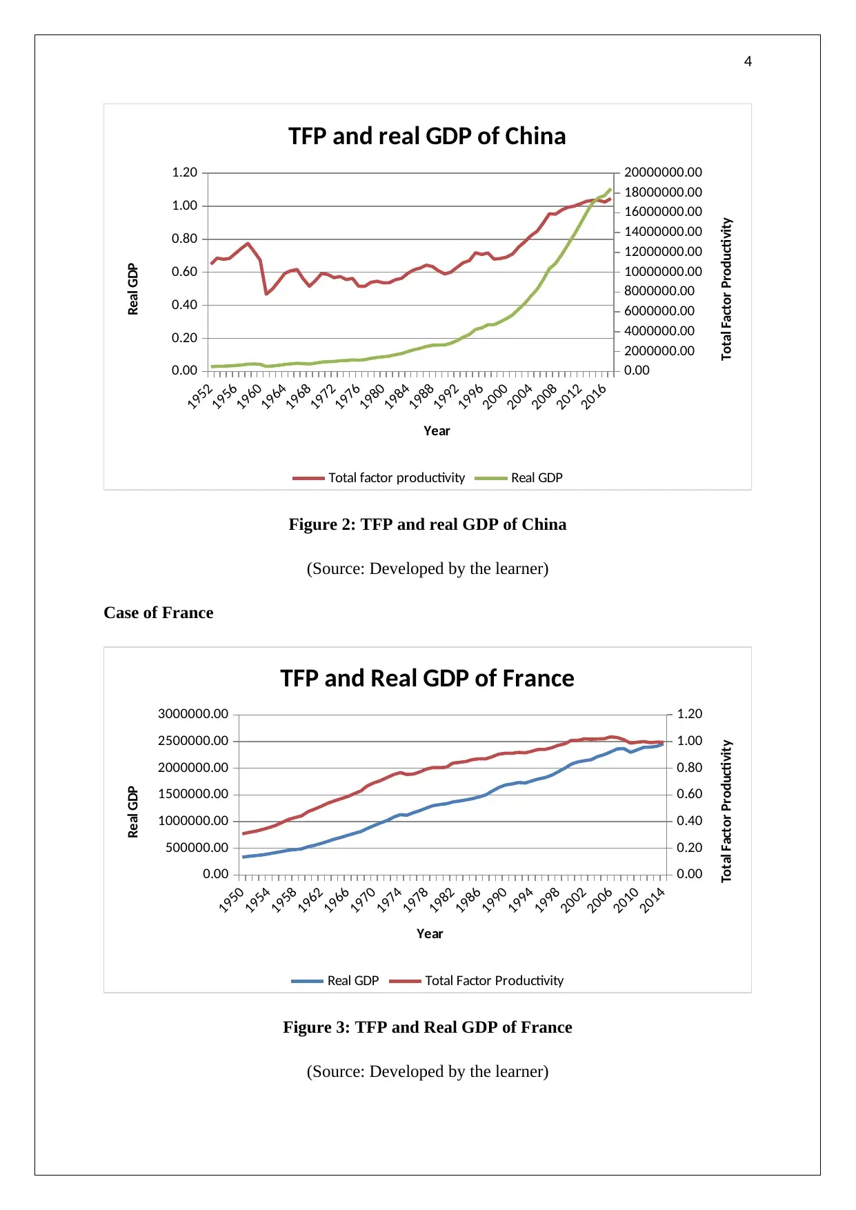
Figure 2: TFP and real GDP of China
(Source: Developed by the learner)
Case of France
1950
1954
1958
1962
1966
1970
1974
1978
1982
1986
1990
1994
1998
2002
2006
2010
2014
0.00
500000.00
1000000.00
1500000.00
2000000.00
2500000.00
3000000.00
0.00
0.20
0.40
0.60
0.80
1.00
1.20
TFP and Real GDP of France
Real GDP Total Factor Productivity
Year
Real GDP
Total Factor Productivity
Figure 3: TFP and Real GDP of France
(Source: Developed by the learner)
1952
1956
1960
1964
1968
1972
1976
1980
1984
1988
1992
1996
2000
2004
2008
2012
2016
0.00
0.20
0.40
0.60
0.80
1.00
1.20
0.00
2000000.00
4000000.00
6000000.00
8000000.00
10000000.00
12000000.00
14000000.00
16000000.00
18000000.00
20000000.00
TFP and real GDP of China
Total factor productivity Real GDP
Year
Real GDP
Total Factor Productivity
Figure 2: TFP and real GDP of China
(Source: Developed by the learner)
Case of France
1950
1954
1958
1962
1966
1970
1974
1978
1982
1986
1990
1994
1998
2002
2006
2010
2014
0.00
500000.00
1000000.00
1500000.00
2000000.00
2500000.00
3000000.00
0.00
0.20
0.40
0.60
0.80
1.00
1.20
TFP and Real GDP of France
Real GDP Total Factor Productivity
Year
Real GDP
Total Factor Productivity
Figure 3: TFP and Real GDP of France
(Source: Developed by the learner)
Paraphrase This Document
Need a fresh take? Get an instant paraphrase of this document with our AI Paraphraser
5
Case of Germany
1950
1954
1958
1962
1966
1970
1974
1978
1982
1986
1990
1994
1998
2002
2006
2010
2014
0.00
500000.00
1000000.00
1500000.00
2000000.00
2500000.00
3000000.00
3500000.00
4000000.00
0.00
0.20
0.40
0.60
0.80
1.00
1.20
TFP and Real GDP of Germany
Real GDP Total Factor Productivity
Year
Real GDP
Total Factor Productivity
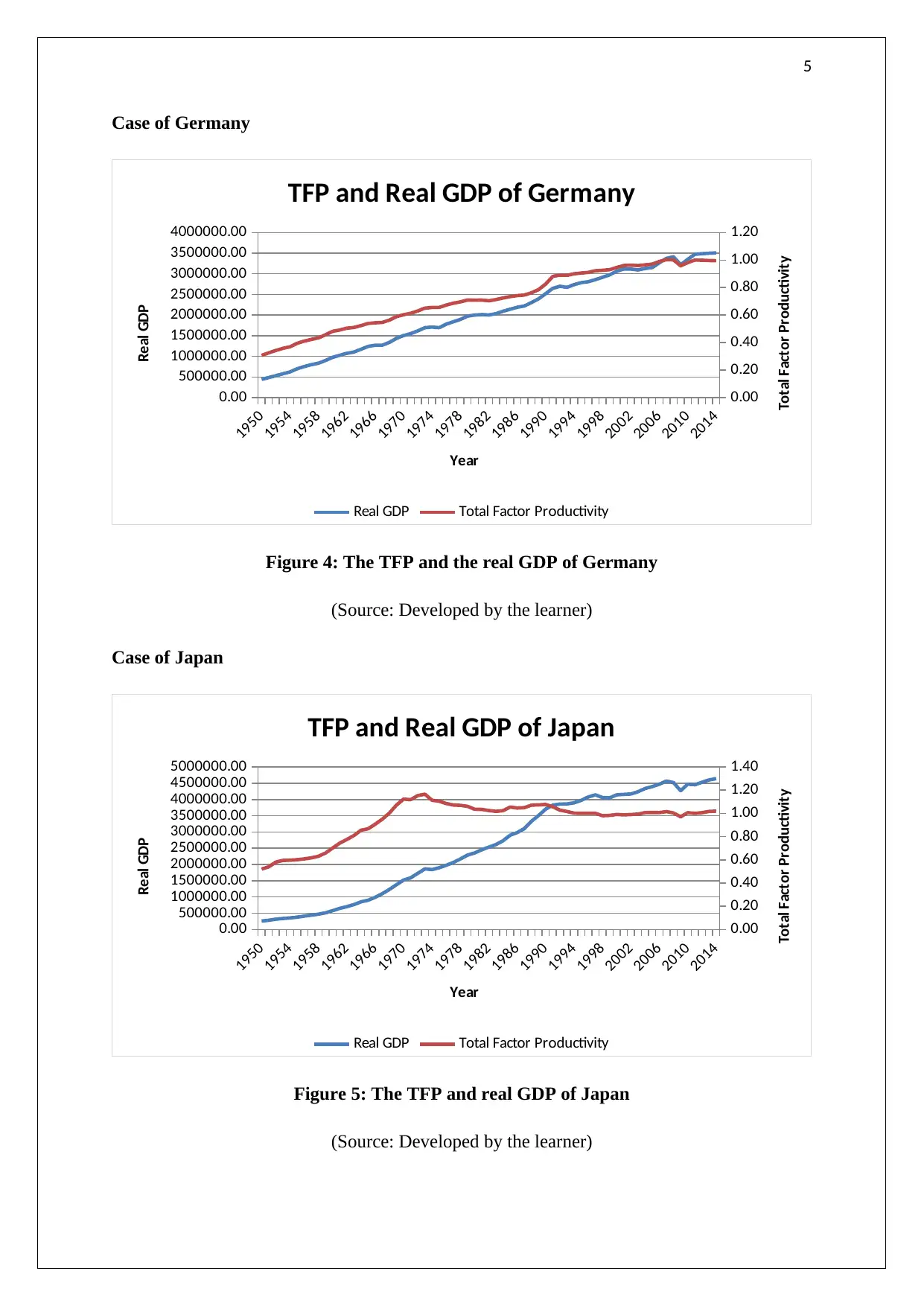
Figure 4: The TFP and the real GDP of Germany
(Source: Developed by the learner)
Case of Japan
1950
1954
1958
1962
1966
1970
1974
1978
1982
1986
1990
1994
1998
2002
2006
2010
2014
0.00
500000.00
1000000.00
1500000.00
2000000.00
2500000.00
3000000.00
3500000.00
4000000.00
4500000.00
5000000.00
0.00
0.20
0.40
0.60
0.80
1.00
1.20
1.40
TFP and Real GDP of Japan
Real GDP Total Factor Productivity
Year
Real GDP
Total Factor Productivity
Figure 5: The TFP and real GDP of Japan
(Source: Developed by the learner)
Case of Germany
1950
1954
1958
1962
1966
1970
1974
1978
1982
1986
1990
1994
1998
2002
2006
2010
2014
0.00
500000.00
1000000.00
1500000.00
2000000.00
2500000.00
3000000.00
3500000.00
4000000.00
0.00
0.20
0.40
0.60
0.80
1.00
1.20
TFP and Real GDP of Germany
Real GDP Total Factor Productivity
Year
Real GDP
Total Factor Productivity
Figure 4: The TFP and the real GDP of Germany
(Source: Developed by the learner)
Case of Japan
1950
1954
1958
1962
1966
1970
1974
1978
1982
1986
1990
1994
1998
2002
2006
2010
2014
0.00
500000.00
1000000.00
1500000.00
2000000.00
2500000.00
3000000.00
3500000.00
4000000.00
4500000.00
5000000.00
0.00
0.20
0.40
0.60
0.80
1.00
1.20
1.40
TFP and Real GDP of Japan
Real GDP Total Factor Productivity
Year
Real GDP
Total Factor Productivity
Figure 5: The TFP and real GDP of Japan
(Source: Developed by the learner)
6
Case of Spain
1950
1954
1958
1962
1966
1970
1974
1978
1982
1986
1990
1994
1998
2002
2006
2010
2014
0.00
200,000.00
400,000.00
600,000.00
800,000.00
1,000,000.00
1,200,000.00
1,400,000.00
1,600,000.00
1,800,000.00
0.00
0.20
0.40
0.60
0.80
1.00
1.20
TFP and real GDP of Spain
Real GDP Total Factor Productivity
Year
Real GDP
Total Factor Productivity
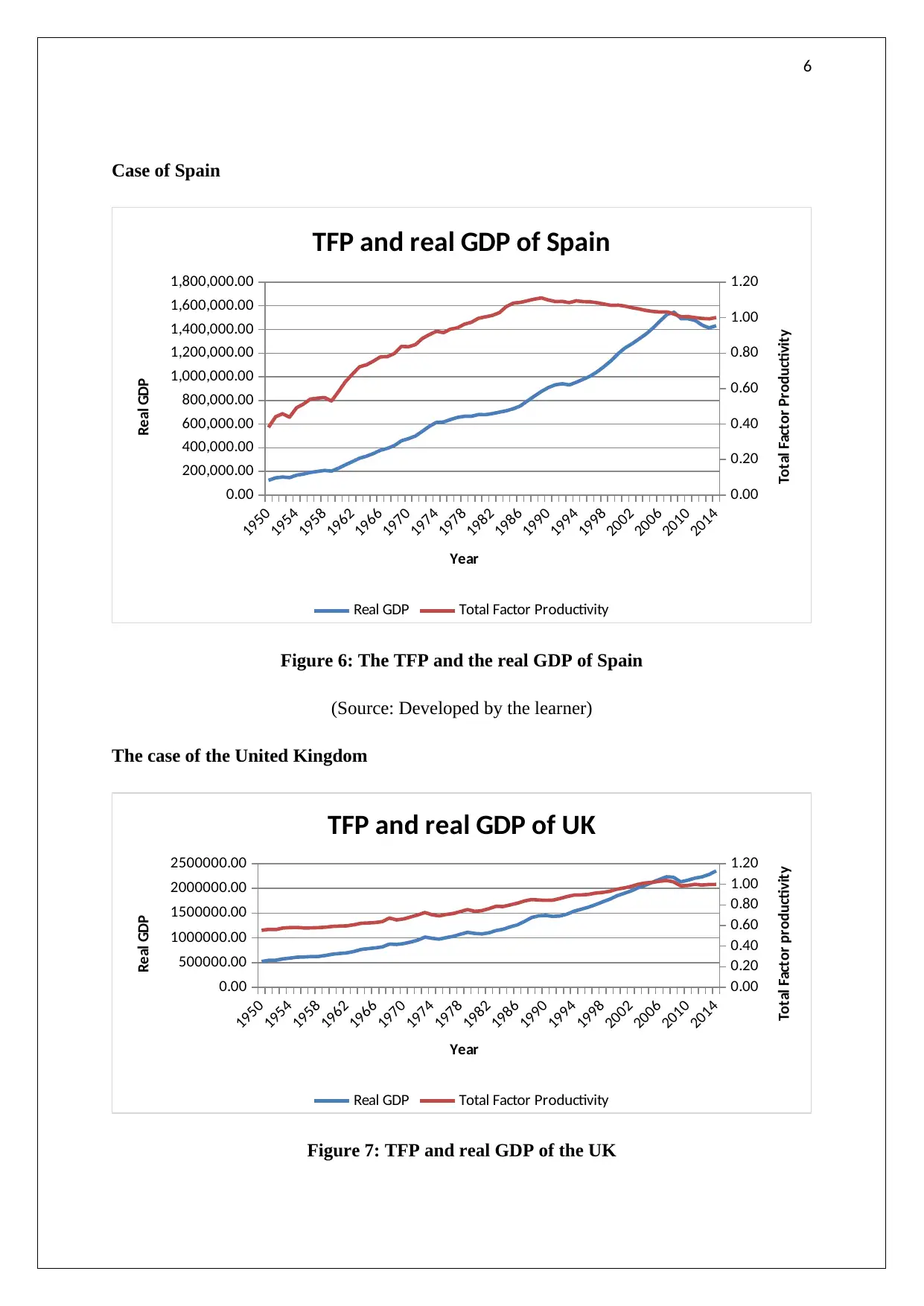
Figure 6: The TFP and the real GDP of Spain
(Source: Developed by the learner)
The case of the United Kingdom
1950
1954
1958
1962
1966
1970
1974
1978
1982
1986
1990
1994
1998
2002
2006
2010
2014
0.00
500000.00
1000000.00
1500000.00
2000000.00
2500000.00
0.00
0.20
0.40
0.60
0.80
1.00
1.20
TFP and real GDP of UK
Real GDP Total Factor Productivity
Year
Real GDP
Total Factor productivity
Figure 7: TFP and real GDP of the UK
Case of Spain
1950
1954
1958
1962
1966
1970
1974
1978
1982
1986
1990
1994
1998
2002
2006
2010
2014
0.00
200,000.00
400,000.00
600,000.00
800,000.00
1,000,000.00
1,200,000.00
1,400,000.00
1,600,000.00
1,800,000.00
0.00
0.20
0.40
0.60
0.80
1.00
1.20
TFP and real GDP of Spain
Real GDP Total Factor Productivity
Year
Real GDP
Total Factor Productivity
Figure 6: The TFP and the real GDP of Spain
(Source: Developed by the learner)
The case of the United Kingdom
1950
1954
1958
1962
1966
1970
1974
1978
1982
1986
1990
1994
1998
2002
2006
2010
2014
0.00
500000.00
1000000.00
1500000.00
2000000.00
2500000.00
0.00
0.20
0.40
0.60
0.80
1.00
1.20
TFP and real GDP of UK
Real GDP Total Factor Productivity
Year
Real GDP
Total Factor productivity
Figure 7: TFP and real GDP of the UK
⊘ This is a preview!⊘
Do you want full access?
Subscribe today to unlock all pages.
Trusted by 1+ million students worldwide
7
(Source: Developed by the learner)
The case of the USA
1950
1954
1958
1962
1966
1970
1974
1978
1982
1986
1990
1994
1998
2002
2006
2010
2014
0.00
2000000.00
4000000.00
6000000.00
8000000.00
10000000.00
12000000.00
14000000.00
16000000.00
18000000.00
0.00
0.20
0.40
0.60
0.80
1.00
1.20
TFP and real GDP of the USA
Real GDP Total Factor Productivity
year
Real GDP
Total Factor Productivity
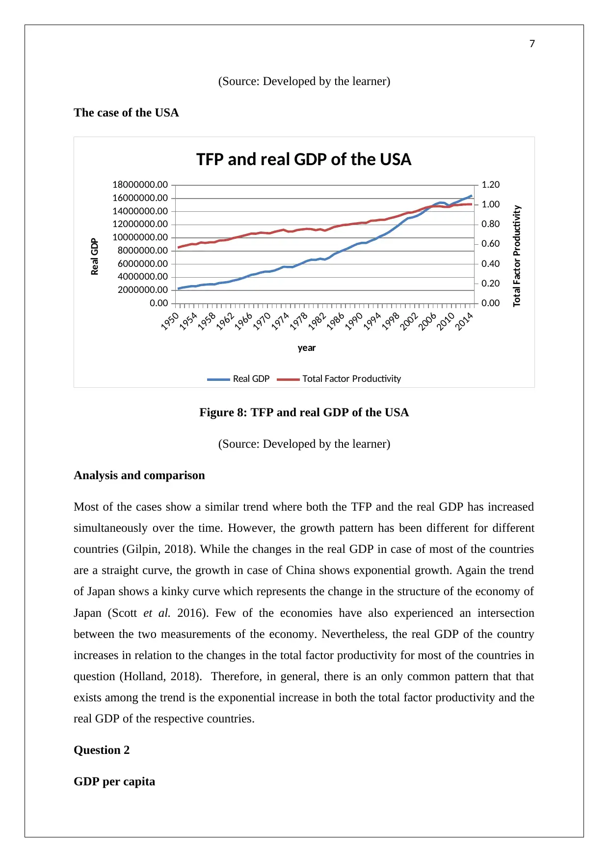
Figure 8: TFP and real GDP of the USA
(Source: Developed by the learner)
Analysis and comparison
Most of the cases show a similar trend where both the TFP and the real GDP has increased
simultaneously over the time. However, the growth pattern has been different for different
countries (Gilpin, 2018). While the changes in the real GDP in case of most of the countries
are a straight curve, the growth in case of China shows exponential growth. Again the trend
of Japan shows a kinky curve which represents the change in the structure of the economy of
Japan (Scott et al. 2016). Few of the economies have also experienced an intersection
between the two measurements of the economy. Nevertheless, the real GDP of the country
increases in relation to the changes in the total factor productivity for most of the countries in
question (Holland, 2018). Therefore, in general, there is an only common pattern that that
exists among the trend is the exponential increase in both the total factor productivity and the
real GDP of the respective countries.
Question 2
GDP per capita
(Source: Developed by the learner)
The case of the USA
1950
1954
1958
1962
1966
1970
1974
1978
1982
1986
1990
1994
1998
2002
2006
2010
2014
0.00
2000000.00
4000000.00
6000000.00
8000000.00
10000000.00
12000000.00
14000000.00
16000000.00
18000000.00
0.00
0.20
0.40
0.60
0.80
1.00
1.20
TFP and real GDP of the USA
Real GDP Total Factor Productivity
year
Real GDP
Total Factor Productivity
Figure 8: TFP and real GDP of the USA
(Source: Developed by the learner)
Analysis and comparison
Most of the cases show a similar trend where both the TFP and the real GDP has increased
simultaneously over the time. However, the growth pattern has been different for different
countries (Gilpin, 2018). While the changes in the real GDP in case of most of the countries
are a straight curve, the growth in case of China shows exponential growth. Again the trend
of Japan shows a kinky curve which represents the change in the structure of the economy of
Japan (Scott et al. 2016). Few of the economies have also experienced an intersection
between the two measurements of the economy. Nevertheless, the real GDP of the country
increases in relation to the changes in the total factor productivity for most of the countries in
question (Holland, 2018). Therefore, in general, there is an only common pattern that that
exists among the trend is the exponential increase in both the total factor productivity and the
real GDP of the respective countries.
Question 2
GDP per capita
Paraphrase This Document
Need a fresh take? Get an instant paraphrase of this document with our AI Paraphraser
8
Year Australia France Japan Germany
2000.0
0 44313.32 38460.68 42169.73 42169.73
2001.0
0 44564.98 38928.03 42239.18 42239.18
2002.0
0 45786.64 39078.20 42190.80 42190.80
2003.0
0 46575.42 39120.20 42744.01 42744.01
2004.0
0 47880.61 39915.26 43671.68 43671.68
2005.0
0 48760.36 40252.42 44393.63 44393.63
2006.0
0 49408.05 40922.08 44995.49 44995.49
2007.0
0 50955.06 41630.09 45687.27 45687.27
2008.0
0 51770.91 41478.94 45165.79 45165.79
2009.0
0 51689.91 40052.31 42724.76 42724.76
2010.0
0 51936.89 40638.33 44507.68 44507.68
2011.0
0 52475.66 41283.15 44538.73 44538.73
2012.0
0 53553.23 41158.88 45276.87 45276.87
2013.0
0 54008.71 41183.51 46249.21 46249.21
2014.0
0 54546.20 41374.76 46484.16 46484.16
2015.0
0 55017.25 41642.31 47163.49 47163.49
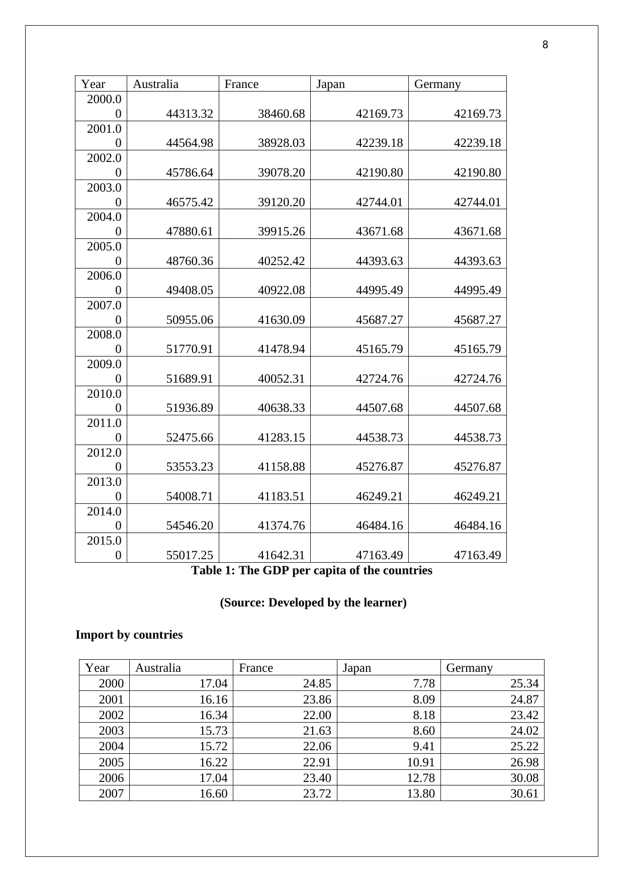
Table 1: The GDP per capita of the countries
(Source: Developed by the learner)
Import by countries
Year Australia France Japan Germany
2000 17.04 24.85 7.78 25.34
2001 16.16 23.86 8.09 24.87
2002 16.34 22.00 8.18 23.42
2003 15.73 21.63 8.60 24.02
2004 15.72 22.06 9.41 25.22
2005 16.22 22.91 10.91 26.98
2006 17.04 23.40 12.78 30.08
2007 16.60 23.72 13.80 30.61
Year Australia France Japan Germany
2000.0
0 44313.32 38460.68 42169.73 42169.73
2001.0
0 44564.98 38928.03 42239.18 42239.18
2002.0
0 45786.64 39078.20 42190.80 42190.80
2003.0
0 46575.42 39120.20 42744.01 42744.01
2004.0
0 47880.61 39915.26 43671.68 43671.68
2005.0
0 48760.36 40252.42 44393.63 44393.63
2006.0
0 49408.05 40922.08 44995.49 44995.49
2007.0
0 50955.06 41630.09 45687.27 45687.27
2008.0
0 51770.91 41478.94 45165.79 45165.79
2009.0
0 51689.91 40052.31 42724.76 42724.76
2010.0
0 51936.89 40638.33 44507.68 44507.68
2011.0
0 52475.66 41283.15 44538.73 44538.73
2012.0
0 53553.23 41158.88 45276.87 45276.87
2013.0
0 54008.71 41183.51 46249.21 46249.21
2014.0
0 54546.20 41374.76 46484.16 46484.16
2015.0
0 55017.25 41642.31 47163.49 47163.49
Table 1: The GDP per capita of the countries
(Source: Developed by the learner)
Import by countries
Year Australia France Japan Germany
2000 17.04 24.85 7.78 25.34
2001 16.16 23.86 8.09 24.87
2002 16.34 22.00 8.18 23.42
2003 15.73 21.63 8.60 24.02
2004 15.72 22.06 9.41 25.22
2005 16.22 22.91 10.91 26.98
2006 17.04 23.40 12.78 30.08
2007 16.60 23.72 13.80 30.61
9
2008 18.18 24.39 15.18 31.41
2009 15.90 20.87 10.51 26.92
2010 15.44 22.97 12.14 30.67
2011 15.47 25.09 13.89 33.18
2012 15.97 25.11 14.24 32.56
2013 15.34 24.34 16.12 31.42
2014 15.65 23.82 16.69 30.86
2015 16.25 23.56 14.74 30.97
2016 14.96 23.21 12.26 30.08
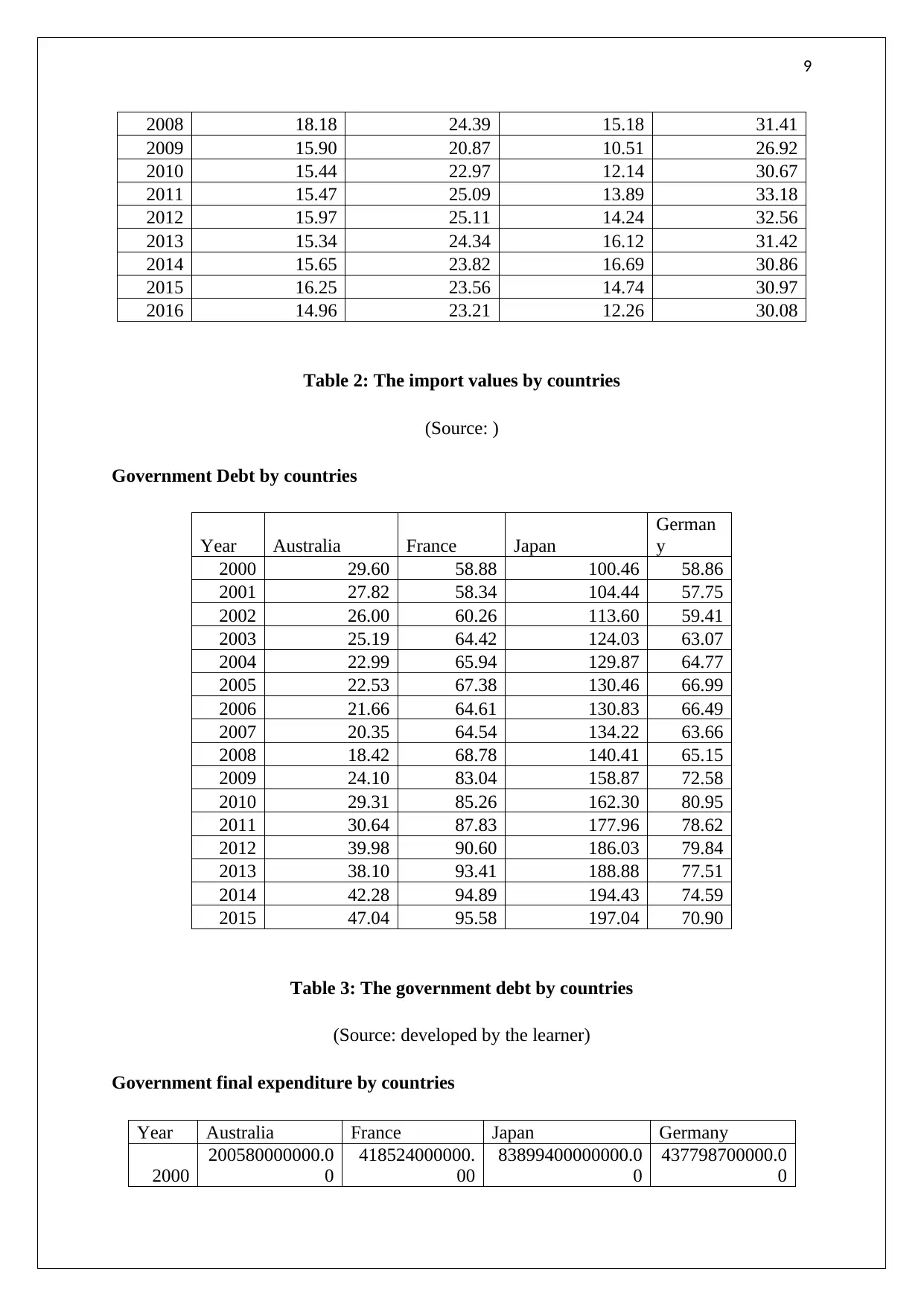
Table 2: The import values by countries
(Source: )
Government Debt by countries
Year Australia France Japan
German
y
2000 29.60 58.88 100.46 58.86
2001 27.82 58.34 104.44 57.75
2002 26.00 60.26 113.60 59.41
2003 25.19 64.42 124.03 63.07
2004 22.99 65.94 129.87 64.77
2005 22.53 67.38 130.46 66.99
2006 21.66 64.61 130.83 66.49
2007 20.35 64.54 134.22 63.66
2008 18.42 68.78 140.41 65.15
2009 24.10 83.04 158.87 72.58
2010 29.31 85.26 162.30 80.95
2011 30.64 87.83 177.96 78.62
2012 39.98 90.60 186.03 79.84
2013 38.10 93.41 188.88 77.51
2014 42.28 94.89 194.43 74.59
2015 47.04 95.58 197.04 70.90
Table 3: The government debt by countries
(Source: developed by the learner)
Government final expenditure by countries
Year Australia France Japan Germany
2000
200580000000.0
0
418524000000.
00
83899400000000.0
0
437798700000.0
0
2008 18.18 24.39 15.18 31.41
2009 15.90 20.87 10.51 26.92
2010 15.44 22.97 12.14 30.67
2011 15.47 25.09 13.89 33.18
2012 15.97 25.11 14.24 32.56
2013 15.34 24.34 16.12 31.42
2014 15.65 23.82 16.69 30.86
2015 16.25 23.56 14.74 30.97
2016 14.96 23.21 12.26 30.08
Table 2: The import values by countries
(Source: )
Government Debt by countries
Year Australia France Japan
German
y
2000 29.60 58.88 100.46 58.86
2001 27.82 58.34 104.44 57.75
2002 26.00 60.26 113.60 59.41
2003 25.19 64.42 124.03 63.07
2004 22.99 65.94 129.87 64.77
2005 22.53 67.38 130.46 66.99
2006 21.66 64.61 130.83 66.49
2007 20.35 64.54 134.22 63.66
2008 18.42 68.78 140.41 65.15
2009 24.10 83.04 158.87 72.58
2010 29.31 85.26 162.30 80.95
2011 30.64 87.83 177.96 78.62
2012 39.98 90.60 186.03 79.84
2013 38.10 93.41 188.88 77.51
2014 42.28 94.89 194.43 74.59
2015 47.04 95.58 197.04 70.90
Table 3: The government debt by countries
(Source: developed by the learner)
Government final expenditure by countries
Year Australia France Japan Germany
2000
200580000000.0
0
418524000000.
00
83899400000000.0
0
437798700000.0
0
⊘ This is a preview!⊘
Do you want full access?
Subscribe today to unlock all pages.
Trusted by 1+ million students worldwide
10
2001
204860000000.0
0
422854000000.
00
86760000000000.0
0
440043370000.0
0
2002 208934000000.0
0
430462000000.
00
89061900000000.0
0
445334410000.0
0
2003 219511000000.0
0
438778000000.
00
90709000000000.0
0
447776420000.0
0
2004 227255000000.0
0
448349000000.
00
91776100000000.0
0
444224410000.0
0
2005 234178000000.0
0
454011000000.
00
92505000000000.0
0
446370420000.0
0
2006 242452000000.0
0
460108000000.
00
92567200000000.0
0
450674760000.0
0
2007 248355000000.0
0
468472000000.
00
93635500000000.0
0
457273140000.0
0
2008 258692000000.0
0
473796000000.
00
93561600000000.0
0
472788560000.0
0
2009 264920000000.0
0
485207000000.
00
95472300000000.0
0
487021300000.0
0
2010 271855000000.0
0
491420000000.
00
97323800000000.0
0
493336000000.0
0
2011 283507000000.0
0
496592000000.
00
99204600000000.0
0
497961020000.0
0
2012 287703000000.0
0
504532000000.
00
100869000000000.
00
503202730000.0
0
2013 291900000000.0
0
511967000000.
00
102382200000000.
00
510010760000.0
0
2014 293823000000.0
0
518650000000.
00
102937600000000.
00
517965810000.0
0
2015 305274000000.0
0
523869000000.
00
104524000000000.
00
533160550000.0
0
2016 321026000000.0
0
531063000000.
00
105914000000000.
00
554225990000.0
0
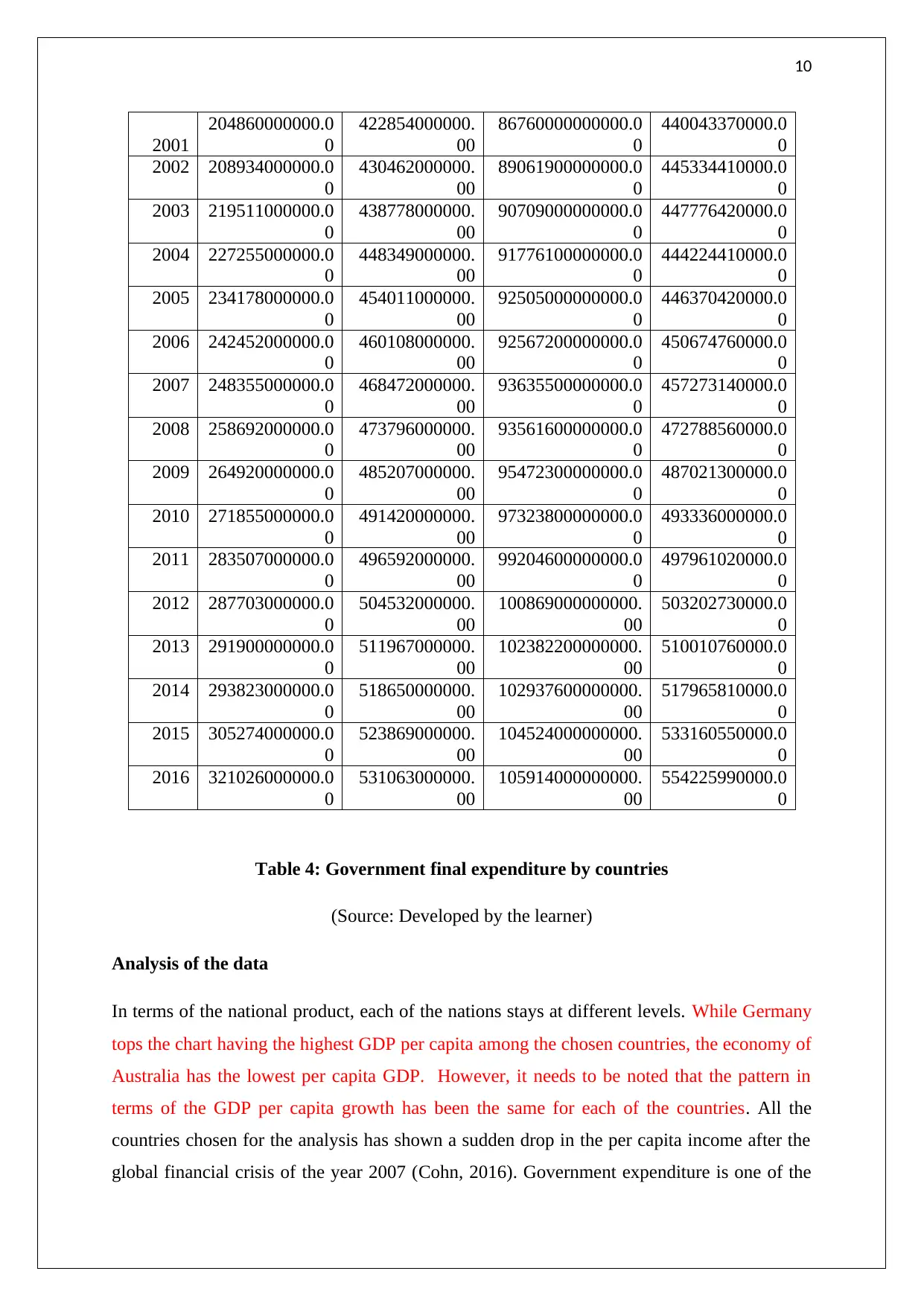
Table 4: Government final expenditure by countries
(Source: Developed by the learner)
Analysis of the data
In terms of the national product, each of the nations stays at different levels. While Germany
tops the chart having the highest GDP per capita among the chosen countries, the economy of
Australia has the lowest per capita GDP. However, it needs to be noted that the pattern in
terms of the GDP per capita growth has been the same for each of the countries. All the
countries chosen for the analysis has shown a sudden drop in the per capita income after the
global financial crisis of the year 2007 (Cohn, 2016). Government expenditure is one of the
2001
204860000000.0
0
422854000000.
00
86760000000000.0
0
440043370000.0
0
2002 208934000000.0
0
430462000000.
00
89061900000000.0
0
445334410000.0
0
2003 219511000000.0
0
438778000000.
00
90709000000000.0
0
447776420000.0
0
2004 227255000000.0
0
448349000000.
00
91776100000000.0
0
444224410000.0
0
2005 234178000000.0
0
454011000000.
00
92505000000000.0
0
446370420000.0
0
2006 242452000000.0
0
460108000000.
00
92567200000000.0
0
450674760000.0
0
2007 248355000000.0
0
468472000000.
00
93635500000000.0
0
457273140000.0
0
2008 258692000000.0
0
473796000000.
00
93561600000000.0
0
472788560000.0
0
2009 264920000000.0
0
485207000000.
00
95472300000000.0
0
487021300000.0
0
2010 271855000000.0
0
491420000000.
00
97323800000000.0
0
493336000000.0
0
2011 283507000000.0
0
496592000000.
00
99204600000000.0
0
497961020000.0
0
2012 287703000000.0
0
504532000000.
00
100869000000000.
00
503202730000.0
0
2013 291900000000.0
0
511967000000.
00
102382200000000.
00
510010760000.0
0
2014 293823000000.0
0
518650000000.
00
102937600000000.
00
517965810000.0
0
2015 305274000000.0
0
523869000000.
00
104524000000000.
00
533160550000.0
0
2016 321026000000.0
0
531063000000.
00
105914000000000.
00
554225990000.0
0
Table 4: Government final expenditure by countries
(Source: Developed by the learner)
Analysis of the data
In terms of the national product, each of the nations stays at different levels. While Germany
tops the chart having the highest GDP per capita among the chosen countries, the economy of
Australia has the lowest per capita GDP. However, it needs to be noted that the pattern in
terms of the GDP per capita growth has been the same for each of the countries. All the
countries chosen for the analysis has shown a sudden drop in the per capita income after the
global financial crisis of the year 2007 (Cohn, 2016). Government expenditure is one of the
Paraphrase This Document
Need a fresh take? Get an instant paraphrase of this document with our AI Paraphraser
11
prime measures of the activity of the government. However, it is different for different
economies chosen for the study. Australia's government spending is too low compared to the
other nations. Another important fact is that government spending also follows a similar
pattern and hence the curve coincides in the case of Germany, France, and Japan. The
economy of Australia has also shown a difference in terms of government debt as well (Liu,
Adam and Walker, 2018). The government of the other countries chosen for the analysis has
taken debt from the external market. Japan economy has a huge budget deficit and that
reflects on the external debt that the government has. And in terms of import, Germany ranks
first as it imports the highest as a percentage of its GDP (Sassen, 2016). There has been a
pattern that is followed by all the countries in terms of import which has also dropped during
the financial crisis of the year 2007. France on the other hand showed a strong relation
between the GDP and the government final consumption. The final consumption of the
government is the independent variable that influences the value of the GDP. In the case of
Germany, the high GDP of the economy requires the government to spend a heavy amount on
the economy that increases the final consumption.
Question 3
1980-01-01
1981-10-01
1983-07-01
1985-04-01
1987-01-01
1988-10-01
1990-07-01
1992-04-01
1994-01-01
1995-10-01
1997-07-01
1999-04-01
2001-01-01
2002-10-01
2004-07-01
2006-04-01
2008-01-01
2009-10-01
2011-07-01
2013-04-01
2015-01-01
2016-10-01
0.0
50000.0
100000.0
150000.0
200000.0
250000.0
0.0
2.0
4.0
6.0
8.0
10.0
12.0
14.0
Unfilled job and unemployment australia
Job vacancies Unemployment
years and quarters
Unfilled Job vacancies
Unemployment rate
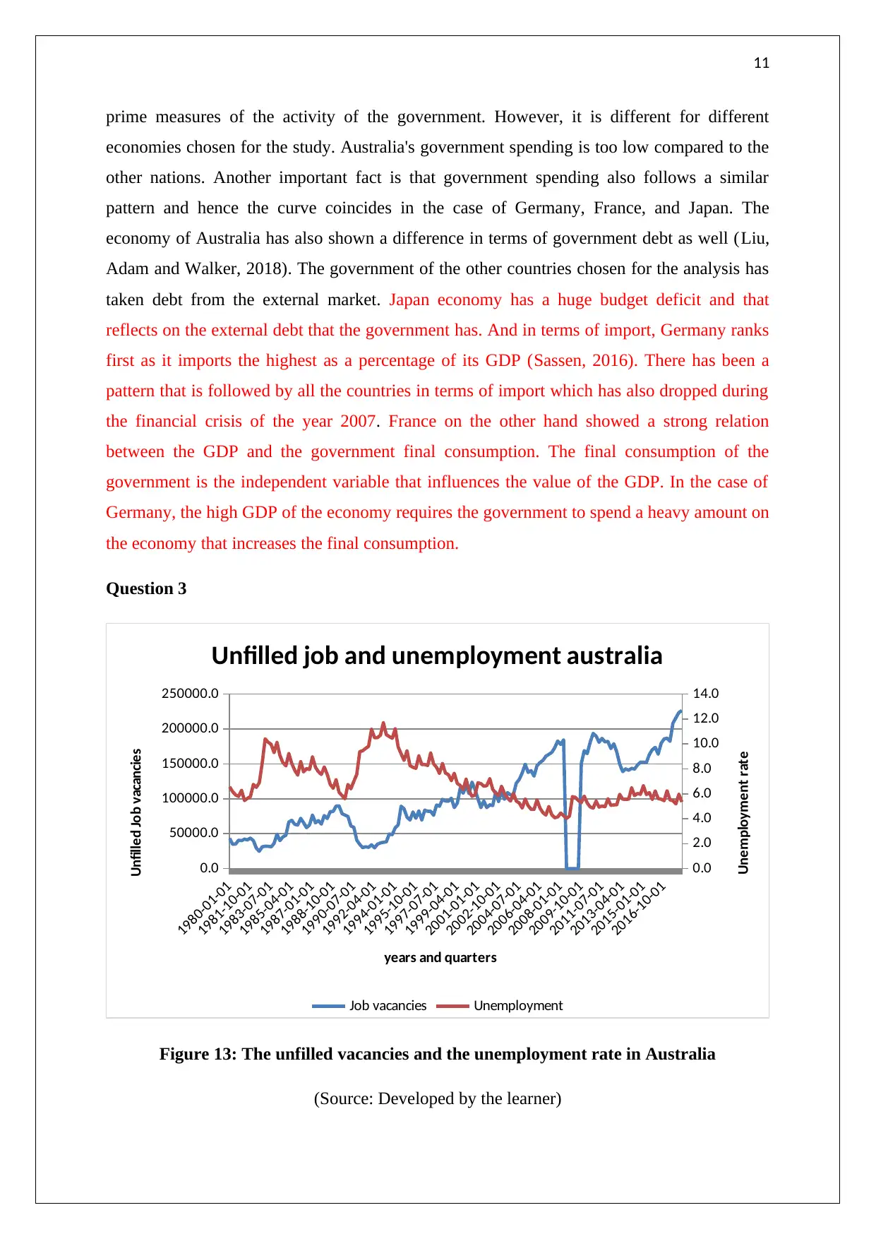
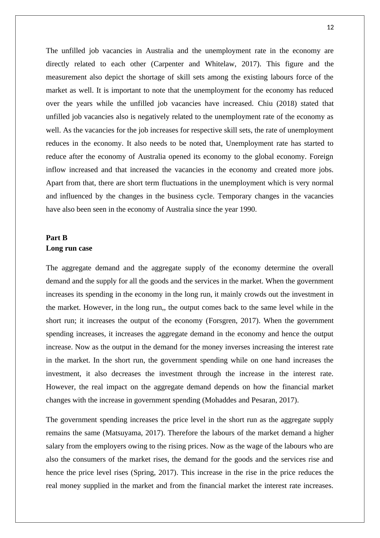
Figure 13: The unfilled vacancies and the unemployment rate in Australia
(Source: Developed by the learner)
prime measures of the activity of the government. However, it is different for different
economies chosen for the study. Australia's government spending is too low compared to the
other nations. Another important fact is that government spending also follows a similar
pattern and hence the curve coincides in the case of Germany, France, and Japan. The
economy of Australia has also shown a difference in terms of government debt as well (Liu,
Adam and Walker, 2018). The government of the other countries chosen for the analysis has
taken debt from the external market. Japan economy has a huge budget deficit and that
reflects on the external debt that the government has. And in terms of import, Germany ranks
first as it imports the highest as a percentage of its GDP (Sassen, 2016). There has been a
pattern that is followed by all the countries in terms of import which has also dropped during
the financial crisis of the year 2007. France on the other hand showed a strong relation
between the GDP and the government final consumption. The final consumption of the
government is the independent variable that influences the value of the GDP. In the case of
Germany, the high GDP of the economy requires the government to spend a heavy amount on
the economy that increases the final consumption.
Question 3
1980-01-01
1981-10-01
1983-07-01
1985-04-01
1987-01-01
1988-10-01
1990-07-01
1992-04-01
1994-01-01
1995-10-01
1997-07-01
1999-04-01
2001-01-01
2002-10-01
2004-07-01
2006-04-01
2008-01-01
2009-10-01
2011-07-01
2013-04-01
2015-01-01
2016-10-01
0.0
50000.0
100000.0
150000.0
200000.0
250000.0
0.0
2.0
4.0
6.0
8.0
10.0
12.0
14.0
Unfilled job and unemployment australia
Job vacancies Unemployment
years and quarters
Unfilled Job vacancies
Unemployment rate
Figure 13: The unfilled vacancies and the unemployment rate in Australia
(Source: Developed by the learner)
12
The unfilled job vacancies in Australia and the unemployment rate in the economy are
directly related to each other (Carpenter and Whitelaw, 2017). This figure and the
measurement also depict the shortage of skill sets among the existing labours force of the
market as well. It is important to note that the unemployment for the economy has reduced
over the years while the unfilled job vacancies have increased. Chiu (2018) stated that
unfilled job vacancies also is negatively related to the unemployment rate of the economy as
well. As the vacancies for the job increases for respective skill sets, the rate of unemployment
reduces in the economy. It also needs to be noted that, Unemployment rate has started to
reduce after the economy of Australia opened its economy to the global economy. Foreign
inflow increased and that increased the vacancies in the economy and created more jobs.
Apart from that, there are short term fluctuations in the unemployment which is very normal
and influenced by the changes in the business cycle. Temporary changes in the vacancies
have also been seen in the economy of Australia since the year 1990.
Part B
Long run case
The aggregate demand and the aggregate supply of the economy determine the overall
demand and the supply for all the goods and the services in the market. When the government
increases its spending in the economy in the long run, it mainly crowds out the investment in
the market. However, in the long run,, the output comes back to the same level while in the
short run; it increases the output of the economy (Forsgren, 2017). When the government
spending increases, it increases the aggregate demand in the economy and hence the output
increase. Now as the output in the demand for the money inverses increasing the interest rate
in the market. In the short run, the government spending while on one hand increases the
investment, it also decreases the investment through the increase in the interest rate.
However, the real impact on the aggregate demand depends on how the financial market
changes with the increase in government spending (Mohaddes and Pesaran, 2017).
The government spending increases the price level in the short run as the aggregate supply
remains the same (Matsuyama, 2017). Therefore the labours of the market demand a higher
salary from the employers owing to the rising prices. Now as the wage of the labours who are
also the consumers of the market rises, the demand for the goods and the services rise and
hence the price level rises (Spring, 2017). This increase in the rise in the price reduces the
real money supplied in the market and from the financial market the interest rate increases.
⊘ This is a preview!⊘
Do you want full access?
Subscribe today to unlock all pages.
Trusted by 1+ million students worldwide
1 out of 17
Related Documents


Your All-in-One AI-Powered Toolkit for Academic Success.
+13062052269
info@desklib.com
Available 24*7 on WhatsApp / Email
![[object Object]](/_next/static/media/star-bottom.7253800d.svg)
Unlock your academic potential
Copyright © 2020–2026 A2Z Services. All Rights Reserved. Developed and managed by ZUCOL.