Study of Global Efforts to Reduce Carbon Emissions: An Analysis
VerifiedAdded on 2022/12/30
|20
|5671
|27
Report
AI Summary
This report provides a comprehensive analysis of carbon emissions and the global efforts to reduce them. The study begins by highlighting the detrimental effects of excessive carbon emissions, including climate change, ozone layer depletion, environmental pollution, and the shrinking of water supplies. It then outlines the methodology, which involves analyzing carbon dioxide data from the Mauna Loa Observatory (1958-2016), employing descriptive statistics like summary analysis and graphical analysis to identify trends and patterns in carbon emissions. The report presents various graphs illustrating the increase in carbon dioxide levels and seasonally adjusted CO2 levels over time. The study emphasizes the significance of its findings for governments, the United Nations, NASA, and the scientific community, offering recommendations for policy development and further research. Overall, the report underscores the urgent need for global cooperation and effective strategies to mitigate the impacts of carbon emissions and promote environmental sustainability.
STUDY OF STEPS TAKEN ALL OVER THE WORLD TO REDUCE EMISSION OF
CARBON
1. Introduction
Carbon emission is a major concern in all parts of the world. Inasmuch as carbon is a very
crucial element in the life of plants and animals, excessive emission of carbon into the
atmosphere is very dangerous. Excessive emission of carbon into the atmosphere is a major
contributor of climate change. Excessive release of carbon causes to the depletion of ozone layer
[1]. Excessive release of carbon also causes pollution of the environment [2].
Excessive emission of carbon into the atmosphere has numerous effects into the environment.
The researchers have proven that excessive emission of carbon into the atmosphere leads to the
shrinking of water supplies [3]. Excessive carbon warms the atmosphere leading to low rainfalls.
Similarly, excessive emission of carbons leads to the reduction of water tables and the pollution
of the water sediments [4]. Therefore, in the long-run, excessive emission of carbon will lead to
the shrinking of water supplies.
Excessive release of carbon causes the increasing incidences of severe weather [5]. Researchers
have demonstrated that excessive release of carbon causes global warming. Global warming
have both direct and indirect severe effects [6]. Apart from directly making severe temperatures
and weather conditions, global warming have associated effects like the typhoons and hurricanes.
The typhoons and hurricanes leads to mass destructions when they occur.
The researchers have also demonstrated that excessive emission of carbon into the atmosphere
leads to drastic changes in the food supply patterns. Excessive emission of carbon into the
atmosphere leads to the change in weather patterns [7]. The changing weather patterns affects the
Paraphrase This Document
Need a fresh take? Get an instant paraphrase of this document with our AI Paraphraser
agricultural industry. The effects include the increase in temperatures and decrease in
precipitations. The decrease in precipitations and increase in temperatures make in unbearable
for the farmers to maintain their foods supply. Therefore, the there is a great need to reduce the
ever- increasing emission of carbon into the atmosphere [8].
The purpose of this study was to find out the steps that can be taken to minimize the release of
carbon [9]. Minimizing the release of carbon was achieved by first studying the patterns of
carbon emission into the atmosphere. The study involved the investigation of the patterns of
carbon emission into the atmosphere from the year 1958 to 2016. The trends of carbon emission
was studied over the period. The study also involved the analysis of association between the
various parameters of carbon emissions. The study of analysis of the association between the
variables was studied through correlation analysis [9]. The study also involved the investigation
of the difference in average carbon emission. Finally, a model that can be used to predict the
amount of carbon emitted into the atmosphere was developed.
The findings and insights from this study will be very significant to a number of stakeholders.
The findings, insights and recommendations will be significant to the governments all over the
world, the United Nations (UN), the National Aeronautics and Space Administration (NASA),
the manufacturing sector and the academicians and researchers in the field of science. The
governments of all countries all over the world can use the findings, insights and
recommendations from this study to establish meaning policies.
The United Nations is responsible for overseeing the environmental practices for various
countries all over the world. Through the United Nations Environmental Program (UNEP), the
United Nations (UN) can use the findings and recommendations from this study to develop
effective policies that are aimed at reducing the rate and magnitude of emission of carbon into
the atmosphere. Moreover, since United Nations (UN) covers a wide range of countries, it can be
the most effective means of developing and enforcing proper environment practice policies [12].
The National Aeronautics and Space Administration (NASA) is responsible for conducting
research on environment and other wide range of areas in the field of science. Therefore, the
findings and insights from this study may add into their existing studies on the environment.
Similarly, the recommendations may form the basis of further research on carbon emission and
global warming. The research can be wide and extensive and hence can lead to the development
of better and effective ways of reducing the emission of carbon into the atmosphere [13].
The researchers and academicians in the field of science may use this study as a reference
material in their work. Similarly, the researchers and academicians in the field of science can use
the recommendations from this study as a basis for further study. Therefore, this research will
contribute immensely to the field of research and science [13].
2. Parameters and the sample population
The data that was used for analysis had five parameters. The study used carbon dioxide record
from Mauna Loa Observatory, known as the “Keeling Curve,” is the world’s longest unbroken
record of atmospheric carbon dioxide concentrations. Scientists make atmospheric measurements
in remote locations to sample air that is representative of a large volume of Earth’s atmosphere
and relatively free from local influences the dataset includes a monthly observation of
atmospheric carbon dioxide (or CO2) concentrations from the Mauna Loa Observatory (Hawaii)
at a latitude of 19.5, longitude of -155.6, and elevation of 3397 meters. The five parameters are
discussed in the paragraph that follows.
⊘ This is a preview!⊘
Do you want full access?
Subscribe today to unlock all pages.
Trusted by 1+ million students worldwide
The first column contained the date parameter. The dates included the months from May 1958 to
October 2016. The second column contained the monthly CO2 concentrations in parts per
million (ppm) measured on the 08A calibration scale and collected at 24:00 hours on the
fifteenth of each month. The third column contained the same data after a seasonal adjustment,
which involves subtracting from the data a 4-harmonic fit with a linear gain factor to remove the
seasonal cycle from carbon dioxide measurements. The fourth column contained the same data
with noise removed, generated from a stiff cubic spline function plus 4-harmonic functions with
linear gain. Finally, the fifth column contained the same data with the seasonal cycle removed.
Data Collection
Data collection techniques are the methods that are used to gather information or data for
analysis. There are numerous techniques of collecting data. A researcher chooses a technique
based on the nature or type of data that is being collected. A data set can be secondary data or
primary data. A primary data consists of the information that is collected on first-hand
information from the field. On the other hand, a secondary data is the information that is
collected from the pre-recorded primary sources [14].
The data that has been used for analysis in this study is a secondary data. Therefore, the data
collection method or technique that was used is secondary. The data was collected from Kaggle
website: https://www.kaggle.com/ucsandiego/carbon-dioxide. The primary data was carbon
dioxide record from Mauna Loa Observatory, known as the “Keeling Curve,” is the world’s
longest unbroken record of atmospheric carbon dioxide concentrations. Scientists make
atmospheric measurements in remote locations to sample air that is representative of a large
volume of Earth’s atmosphere and relatively free from local influences.
Paraphrase This Document
Need a fresh take? Get an instant paraphrase of this document with our AI Paraphraser
The carbon dioxide data was collected and published by the University of California's Scripps
Institution of Oceanography under the supervision of Charles David Keeling with support from
the US Department of Energy, Earth Networks, and the National Science Foundation. The
inspiration of collecting the primary data was to provide answer to a number of questions. Some
of the questions that the researchers sought to answer include: How have atmospheric carbon
dioxide levels changed in the past sixty years? How do carbon dioxide concentrations change
seasonally? What do you think causes this seasonal cycle? When will the carbon dioxide levels
exceed 450 parts per million?
Descriptive statistics
Descriptive analysis is a form of exploratory data analysis. Descriptive analysis was conducted to
establish some of the important features of the variables of the data. The descriptive analyses that
were conducted in this study include the summary analysis and graphical analysis. The results of
analyses are outlined in the sections that follow [13].
Summary Statistics
Summary statistics analysis outlines some of the important features of the data set [12]. The
features that were obtained by summary analysis include: The mean or average, the standard
deviation, the median, the mode, the standard error, the sample variance, the kurtosis, the
skewness, the range, the minimum and the maximum. The results of the parameters are outlined
in the table below.
Carbon
Dioxide
(ppm)
Seasonally
Adjusted CO2
(ppm)
Carbon
Dioxide Fit
(ppm)
Seasonally Adjusted
CO2 Fit (ppm)
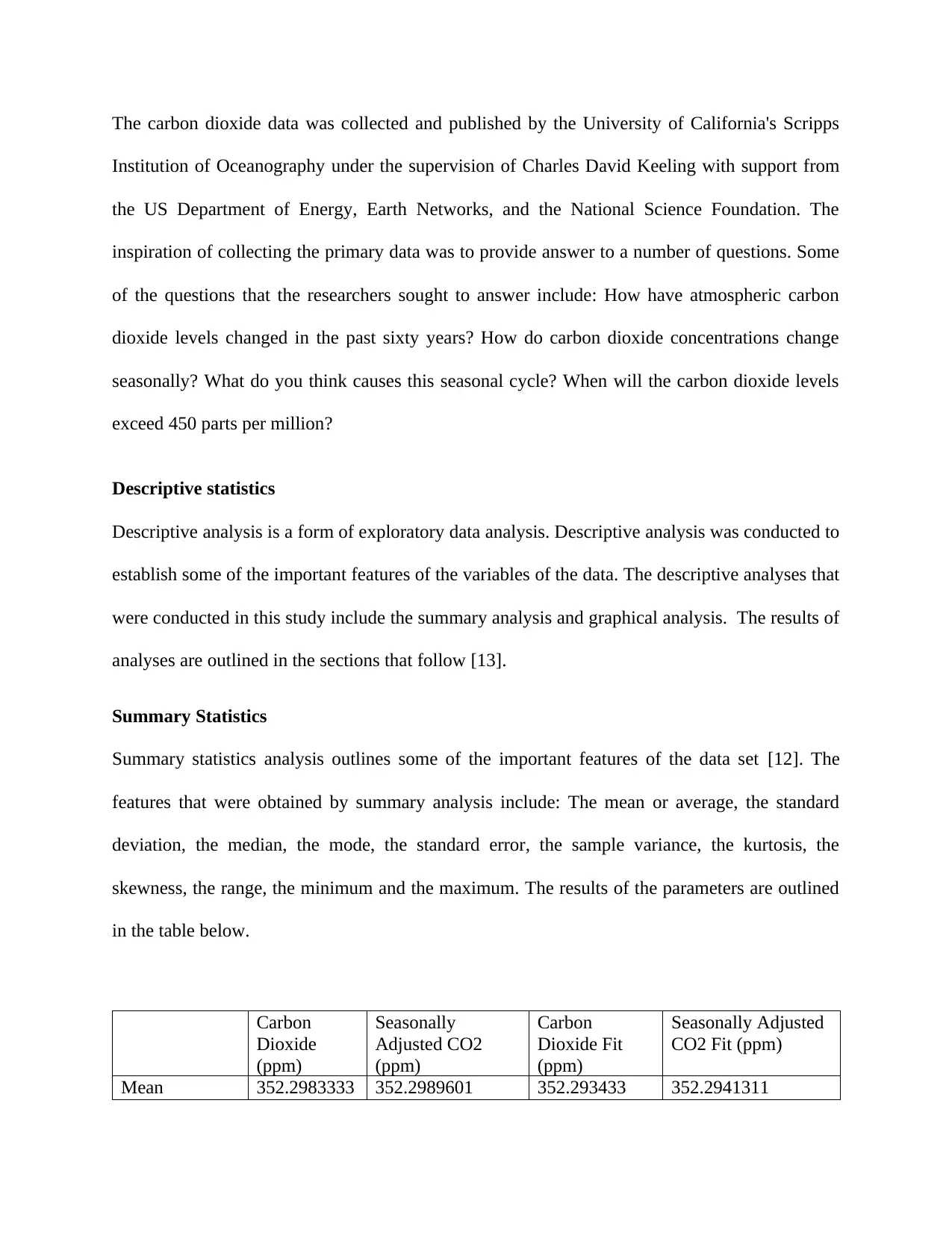
Mean 352.2983333 352.2989601 352.293433 352.2941311
Institution of Oceanography under the supervision of Charles David Keeling with support from
the US Department of Energy, Earth Networks, and the National Science Foundation. The
inspiration of collecting the primary data was to provide answer to a number of questions. Some
of the questions that the researchers sought to answer include: How have atmospheric carbon
dioxide levels changed in the past sixty years? How do carbon dioxide concentrations change
seasonally? What do you think causes this seasonal cycle? When will the carbon dioxide levels
exceed 450 parts per million?
Descriptive statistics
Descriptive analysis is a form of exploratory data analysis. Descriptive analysis was conducted to
establish some of the important features of the variables of the data. The descriptive analyses that
were conducted in this study include the summary analysis and graphical analysis. The results of
analyses are outlined in the sections that follow [13].
Summary Statistics
Summary statistics analysis outlines some of the important features of the data set [12]. The
features that were obtained by summary analysis include: The mean or average, the standard
deviation, the median, the mode, the standard error, the sample variance, the kurtosis, the
skewness, the range, the minimum and the maximum. The results of the parameters are outlined
in the table below.
Carbon
Dioxide
(ppm)
Seasonally
Adjusted CO2
(ppm)
Carbon
Dioxide Fit
(ppm)
Seasonally Adjusted
CO2 Fit (ppm)
Mean 352.2983333 352.2989601 352.293433 352.2941311
Standard Error 0.988114723 0.985535065 0.988056015 0.985466186
Median 349.675 349.74 349.875 349.825
Mode 357.16 319.42 315.71 0
Standard
Deviation
26.18037882 26.11203005 26.17882335 26.11020509
Sample
Variance
685.412235 681.8381132 685.3307918 681.74281
Kurtosis -
1.081255167
-1.090065342 -1.08125025 -1.090727816
Skewness 0.321521946 0.32423533 0.321152187 0.323882216
Range 94.44 91.62 94.8 90.94
Minimum 313.21 314.42 312.48 314.89
Maximum 407.65 406.04 407.28 405.83
Sum 247313.43 247313.87 247309.99 247310.48
Count 702 702 702 702
Confidence
Level (95.0%)
1.940018855 1.934954073 1.939903591 1.934818841
Graphical analysis
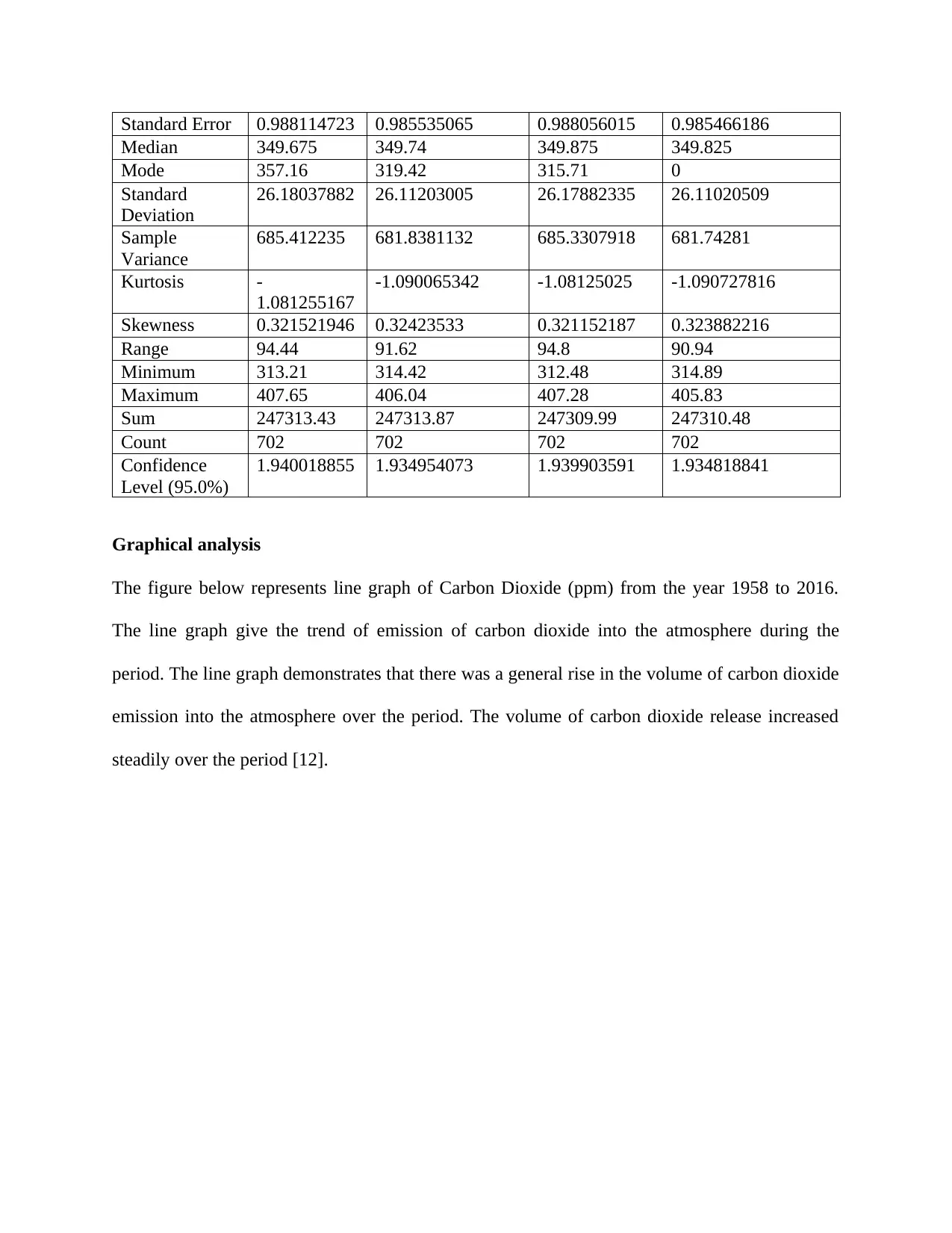
The figure below represents line graph of Carbon Dioxide (ppm) from the year 1958 to 2016.
The line graph give the trend of emission of carbon dioxide into the atmosphere during the
period. The line graph demonstrates that there was a general rise in the volume of carbon dioxide
emission into the atmosphere over the period. The volume of carbon dioxide release increased
steadily over the period [12].
Median 349.675 349.74 349.875 349.825
Mode 357.16 319.42 315.71 0
Standard
Deviation
26.18037882 26.11203005 26.17882335 26.11020509
Sample
Variance
685.412235 681.8381132 685.3307918 681.74281
Kurtosis -
1.081255167
-1.090065342 -1.08125025 -1.090727816
Skewness 0.321521946 0.32423533 0.321152187 0.323882216
Range 94.44 91.62 94.8 90.94
Minimum 313.21 314.42 312.48 314.89
Maximum 407.65 406.04 407.28 405.83
Sum 247313.43 247313.87 247309.99 247310.48
Count 702 702 702 702
Confidence
Level (95.0%)
1.940018855 1.934954073 1.939903591 1.934818841
Graphical analysis
The figure below represents line graph of Carbon Dioxide (ppm) from the year 1958 to 2016.
The line graph give the trend of emission of carbon dioxide into the atmosphere during the
period. The line graph demonstrates that there was a general rise in the volume of carbon dioxide
emission into the atmosphere over the period. The volume of carbon dioxide release increased
steadily over the period [12].
⊘ This is a preview!⊘
Do you want full access?
Subscribe today to unlock all pages.
Trusted by 1+ million students worldwide
May-58
Feb-61
Nov-63
Aug-66
May-69
Feb-72
Nov-74
Aug-77
May-80
Feb-83
Nov-85
Aug-88
May-91
Feb-94
Nov-96
Aug-99
May-02
Feb-05
Nov-07
Aug-10
May-13
Feb-16
0
50
100
150
200
250
300
350
400
450
A Line Graph of Carbon Dioxide (ppm)
Carbon Dioxide (ppm)
Month
Volume
The figure below is a line graph of the seasonally adjusted CO2 (Ppm) over the period between
1958 and 2016. The line graph outlines the trend of the seasonally adjusted CO2 (Ppm) over the
period between 1958 and 2016. The graph demonstrates that there was a consistent increase in
the level of the seasonally adjusted CO2 (Ppm) over the period between 1958 and 2016 [5].
May-58
Jul-61
Sep-64
Nov-67
Jan-71
Mar-74
May-77
Jul-80
Sep-83
Nov-86
Jan-90
Mar-93
May-96
Jul-99
Sep-02
Nov-05
Jan-09
Mar-12
May-15
0
50
100
150
200
250
300
350
400
450
A Line Graph of Seasonally Adjusted CO2 (ppm)
Seasonally Adjusted CO2 (ppm)
Month
Volume
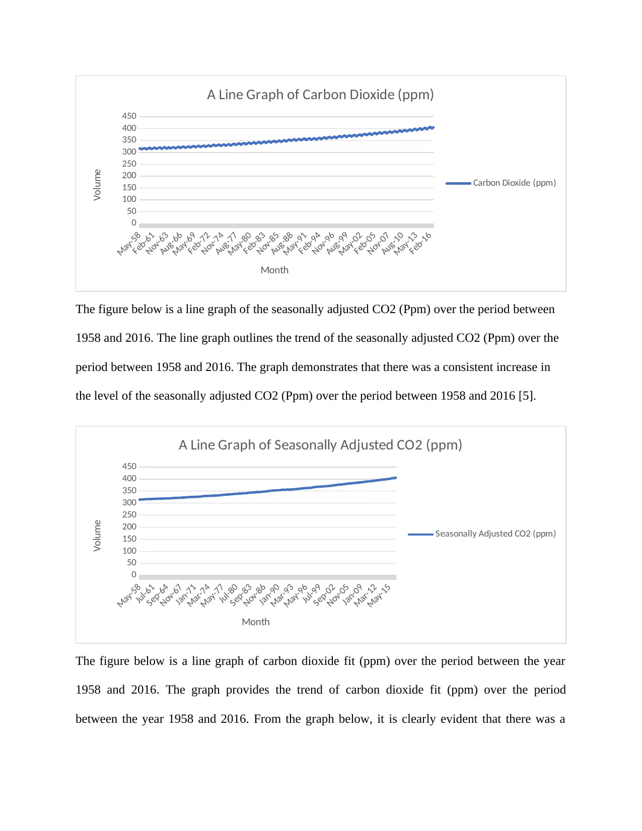
The figure below is a line graph of carbon dioxide fit (ppm) over the period between the year
1958 and 2016. The graph provides the trend of carbon dioxide fit (ppm) over the period
between the year 1958 and 2016. From the graph below, it is clearly evident that there was a
Feb-61
Nov-63
Aug-66
May-69
Feb-72
Nov-74
Aug-77
May-80
Feb-83
Nov-85
Aug-88
May-91
Feb-94
Nov-96
Aug-99
May-02
Feb-05
Nov-07
Aug-10
May-13
Feb-16
0
50
100
150
200
250
300
350
400
450
A Line Graph of Carbon Dioxide (ppm)
Carbon Dioxide (ppm)
Month
Volume
The figure below is a line graph of the seasonally adjusted CO2 (Ppm) over the period between
1958 and 2016. The line graph outlines the trend of the seasonally adjusted CO2 (Ppm) over the
period between 1958 and 2016. The graph demonstrates that there was a consistent increase in
the level of the seasonally adjusted CO2 (Ppm) over the period between 1958 and 2016 [5].
May-58
Jul-61
Sep-64
Nov-67
Jan-71
Mar-74
May-77
Jul-80
Sep-83
Nov-86
Jan-90
Mar-93
May-96
Jul-99
Sep-02
Nov-05
Jan-09
Mar-12
May-15
0
50
100
150
200
250
300
350
400
450
A Line Graph of Seasonally Adjusted CO2 (ppm)
Seasonally Adjusted CO2 (ppm)
Month
Volume
The figure below is a line graph of carbon dioxide fit (ppm) over the period between the year
1958 and 2016. The graph provides the trend of carbon dioxide fit (ppm) over the period
between the year 1958 and 2016. From the graph below, it is clearly evident that there was a
Paraphrase This Document
Need a fresh take? Get an instant paraphrase of this document with our AI Paraphraser
consistent increase in the volume of carbon dioxide fit (ppm) over the period between the year
1958 and 2016 [14].
May-58
Jul-61
Sep-64
Nov-67
Jan-71
Mar-74
May-77
Jul-80
Sep-83
Nov-86
Jan-90
Mar-93
May-96
Jul-99
Sep-02
Nov-05
Jan-09
Mar-12
May-15
0
50
100
150
200
250
300
350
400
450
A Line Graph of Carbon Dioxide Fit (ppm)
Carbon Dioxide Fit (ppm)
Month
Volume
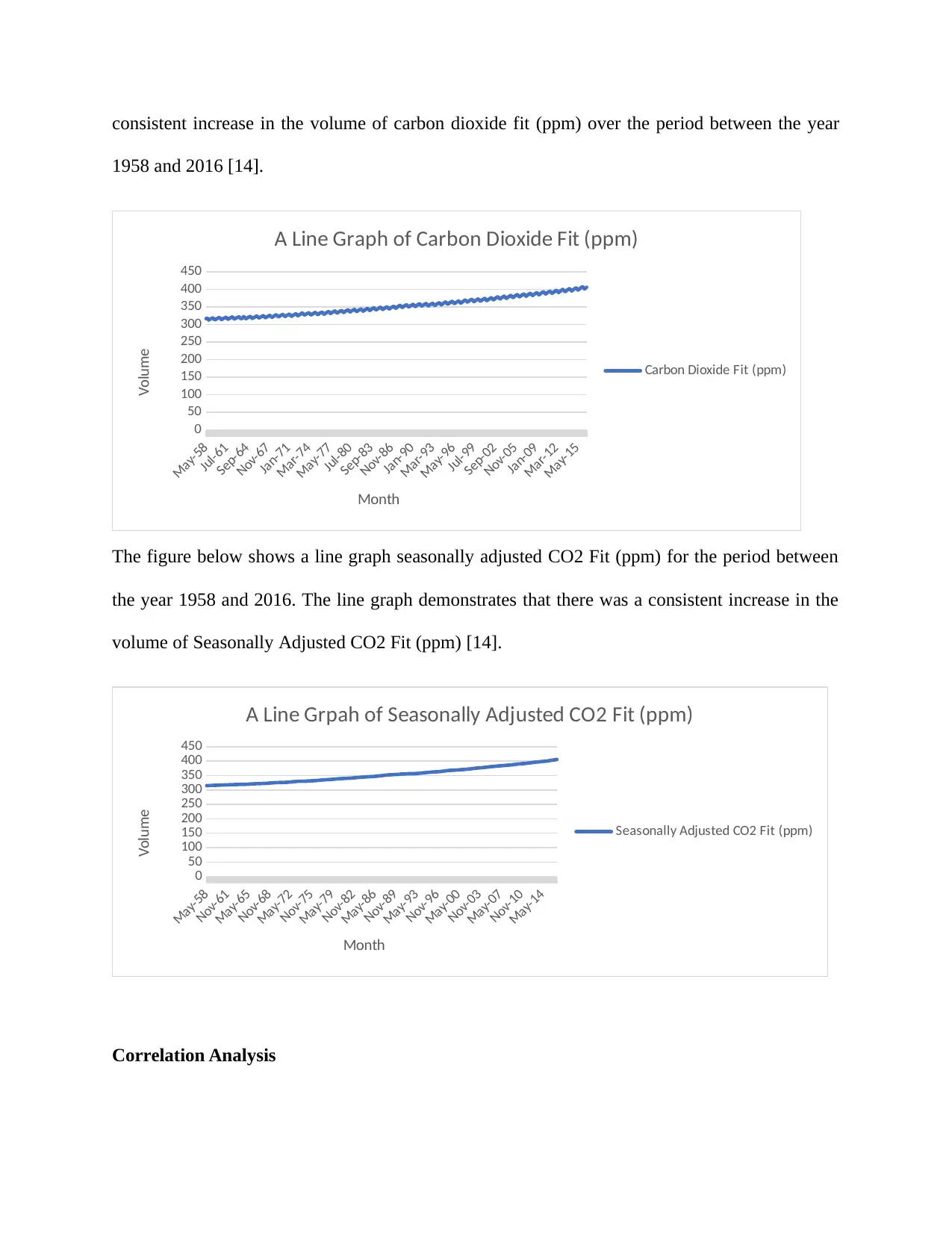
The figure below shows a line graph seasonally adjusted CO2 Fit (ppm) for the period between
the year 1958 and 2016. The line graph demonstrates that there was a consistent increase in the
volume of Seasonally Adjusted CO2 Fit (ppm) [14].
May-58
Nov-61
May-65
Nov-68
May-72
Nov-75
May-79
Nov-82
May-86
Nov-89
May-93
Nov-96
May-00
Nov-03
May-07
Nov-10
May-14
0
50
100
150
200
250
300
350
400
450
A Line Grpah of Seasonally Adjusted CO2 Fit (ppm)
Seasonally Adjusted CO2 Fit (ppm)
Month
Volume
Correlation Analysis
1958 and 2016 [14].
May-58
Jul-61
Sep-64
Nov-67
Jan-71
Mar-74
May-77
Jul-80
Sep-83
Nov-86
Jan-90
Mar-93
May-96
Jul-99
Sep-02
Nov-05
Jan-09
Mar-12
May-15
0
50
100
150
200
250
300
350
400
450
A Line Graph of Carbon Dioxide Fit (ppm)
Carbon Dioxide Fit (ppm)
Month
Volume
The figure below shows a line graph seasonally adjusted CO2 Fit (ppm) for the period between
the year 1958 and 2016. The line graph demonstrates that there was a consistent increase in the
volume of Seasonally Adjusted CO2 Fit (ppm) [14].
May-58
Nov-61
May-65
Nov-68
May-72
Nov-75
May-79
Nov-82
May-86
Nov-89
May-93
Nov-96
May-00
Nov-03
May-07
Nov-10
May-14
0
50
100
150
200
250
300
350
400
450
A Line Grpah of Seasonally Adjusted CO2 Fit (ppm)
Seasonally Adjusted CO2 Fit (ppm)
Month
Volume
Correlation Analysis
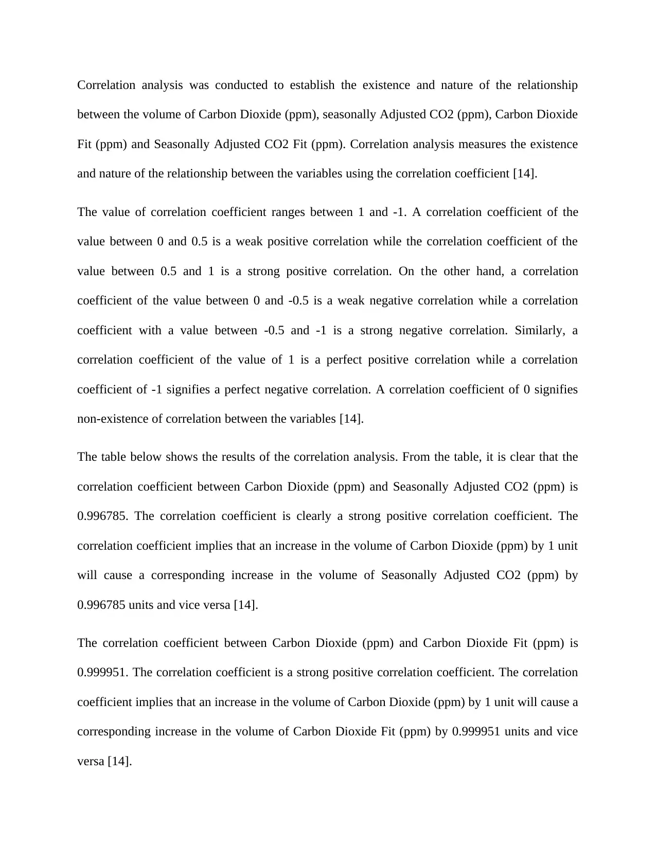
Correlation analysis was conducted to establish the existence and nature of the relationship
between the volume of Carbon Dioxide (ppm), seasonally Adjusted CO2 (ppm), Carbon Dioxide
Fit (ppm) and Seasonally Adjusted CO2 Fit (ppm). Correlation analysis measures the existence
and nature of the relationship between the variables using the correlation coefficient [14].
The value of correlation coefficient ranges between 1 and -1. A correlation coefficient of the
value between 0 and 0.5 is a weak positive correlation while the correlation coefficient of the
value between 0.5 and 1 is a strong positive correlation. On the other hand, a correlation
coefficient of the value between 0 and -0.5 is a weak negative correlation while a correlation
coefficient with a value between -0.5 and -1 is a strong negative correlation. Similarly, a
correlation coefficient of the value of 1 is a perfect positive correlation while a correlation
coefficient of -1 signifies a perfect negative correlation. A correlation coefficient of 0 signifies
non-existence of correlation between the variables [14].
The table below shows the results of the correlation analysis. From the table, it is clear that the
correlation coefficient between Carbon Dioxide (ppm) and Seasonally Adjusted CO2 (ppm) is
0.996785. The correlation coefficient is clearly a strong positive correlation coefficient. The
correlation coefficient implies that an increase in the volume of Carbon Dioxide (ppm) by 1 unit
will cause a corresponding increase in the volume of Seasonally Adjusted CO2 (ppm) by
0.996785 units and vice versa [14].
The correlation coefficient between Carbon Dioxide (ppm) and Carbon Dioxide Fit (ppm) is
0.999951. The correlation coefficient is a strong positive correlation coefficient. The correlation
coefficient implies that an increase in the volume of Carbon Dioxide (ppm) by 1 unit will cause a
corresponding increase in the volume of Carbon Dioxide Fit (ppm) by 0.999951 units and vice
versa [14].
⊘ This is a preview!⊘
Do you want full access?
Subscribe today to unlock all pages.
Trusted by 1+ million students worldwide

The correlation coefficient between Carbon Dioxide (ppm) and Seasonally Adjusted CO2 Fit
(ppm) is 0.996736. The correlation coefficient is a positive correlation coefficient. The
correlation coefficient implies that an increase in the volume of Carbon Dioxide (ppm) by 1 unit
will cause a corresponding increase in the volume of Seasonally Adjusted CO2 Fit (ppm) by
0.996736 units and vice versa [14].
The correlation coefficient between Seasonally Adjusted CO2 (ppm) and Carbon Dioxide Fit
(ppm) is 0.996736. This is a strong positive correlation. The correlation coefficient implies that
an increase in the volume of Seasonally Adjusted CO2 (ppm) by 1 unit will cause a
corresponding increase in the volume of Carbon Dioxide Fit (ppm) by 0.996736 units and vice
versa [14].
The correlation coefficient between Seasonally Adjusted CO2 (ppm) and Seasonally Adjusted
CO2 Fit (ppm) is 0.999951 which is a strong positive correlation coefficient. The correlation
coefficient implies that an increase in the volume of Seasonally Adjusted CO2 (ppm) by 1 unit
will cause a corresponding increase in the volume of Seasonally Adjusted CO2 Fit (ppm) by
0.999951 units and vice versa [14].
The correlation coefficient between Carbon Dioxide Fit (ppm and Seasonally Adjusted CO2 Fit
(ppm) is 0.996784. The correlation coefficient signifies a strong positive correlation coefficient.
The correlation coefficient implies that an increase in the volume of Carbon Dioxide Fit (ppm by
1 unit will cause a corresponding increase in the volume of seasonally Adjusted CO2 Fit (ppm)
by 0.996784 units [14].
Carbon
Dioxide
(ppm)
Seasonally
Adjusted CO2
(ppm)
Carbon
Dioxide Fit
(ppm)
Seasonally
Adjusted CO2 Fit
(ppm)
Carbon Dioxide 1
Paraphrase This Document
Need a fresh take? Get an instant paraphrase of this document with our AI Paraphraser
(ppm)
Seasonally
Adjusted CO2
(ppm)
0.996785 1
Carbon Dioxide Fit
(ppm)
0.999951 0.996736 1
Seasonally
Adjusted CO2 Fit
(ppm)
0.996736 0.999951 0.996784 1
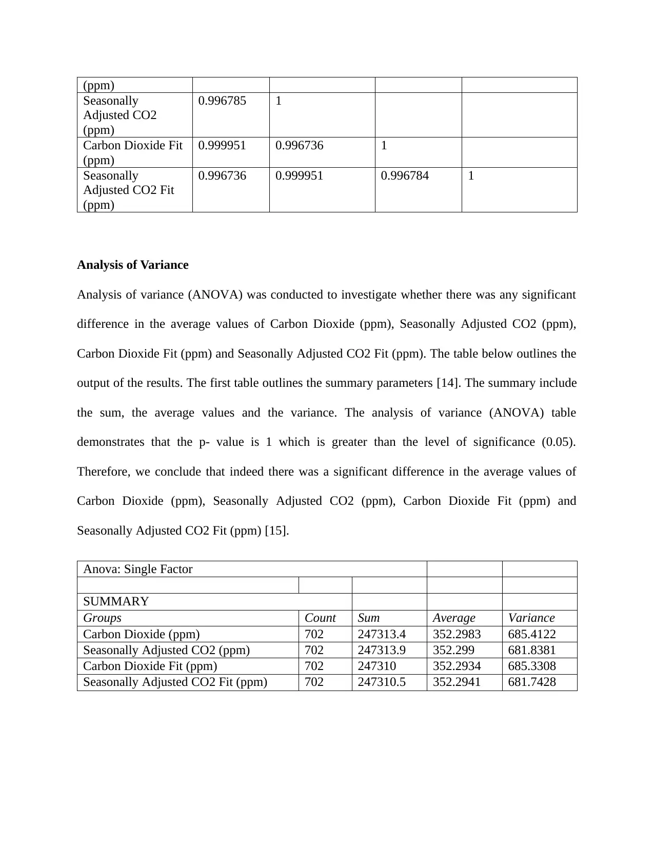
Analysis of Variance
Analysis of variance (ANOVA) was conducted to investigate whether there was any significant
difference in the average values of Carbon Dioxide (ppm), Seasonally Adjusted CO2 (ppm),
Carbon Dioxide Fit (ppm) and Seasonally Adjusted CO2 Fit (ppm). The table below outlines the
output of the results. The first table outlines the summary parameters [14]. The summary include
the sum, the average values and the variance. The analysis of variance (ANOVA) table
demonstrates that the p- value is 1 which is greater than the level of significance (0.05).
Therefore, we conclude that indeed there was a significant difference in the average values of
Carbon Dioxide (ppm), Seasonally Adjusted CO2 (ppm), Carbon Dioxide Fit (ppm) and
Seasonally Adjusted CO2 Fit (ppm) [15].
Anova: Single Factor
SUMMARY
Groups Count Sum Average Variance
Carbon Dioxide (ppm) 702 247313.4 352.2983 685.4122
Seasonally Adjusted CO2 (ppm) 702 247313.9 352.299 681.8381
Carbon Dioxide Fit (ppm) 702 247310 352.2934 685.3308
Seasonally Adjusted CO2 Fit (ppm) 702 247310.5 352.2941 681.7428
Seasonally
Adjusted CO2
(ppm)
0.996785 1
Carbon Dioxide Fit
(ppm)
0.999951 0.996736 1
Seasonally
Adjusted CO2 Fit
(ppm)
0.996736 0.999951 0.996784 1
Analysis of Variance
Analysis of variance (ANOVA) was conducted to investigate whether there was any significant
difference in the average values of Carbon Dioxide (ppm), Seasonally Adjusted CO2 (ppm),
Carbon Dioxide Fit (ppm) and Seasonally Adjusted CO2 Fit (ppm). The table below outlines the
output of the results. The first table outlines the summary parameters [14]. The summary include
the sum, the average values and the variance. The analysis of variance (ANOVA) table
demonstrates that the p- value is 1 which is greater than the level of significance (0.05).
Therefore, we conclude that indeed there was a significant difference in the average values of
Carbon Dioxide (ppm), Seasonally Adjusted CO2 (ppm), Carbon Dioxide Fit (ppm) and
Seasonally Adjusted CO2 Fit (ppm) [15].
Anova: Single Factor
SUMMARY
Groups Count Sum Average Variance
Carbon Dioxide (ppm) 702 247313.4 352.2983 685.4122
Seasonally Adjusted CO2 (ppm) 702 247313.9 352.299 681.8381
Carbon Dioxide Fit (ppm) 702 247310 352.2934 685.3308
Seasonally Adjusted CO2 Fit (ppm) 702 247310.5 352.2941 681.7428
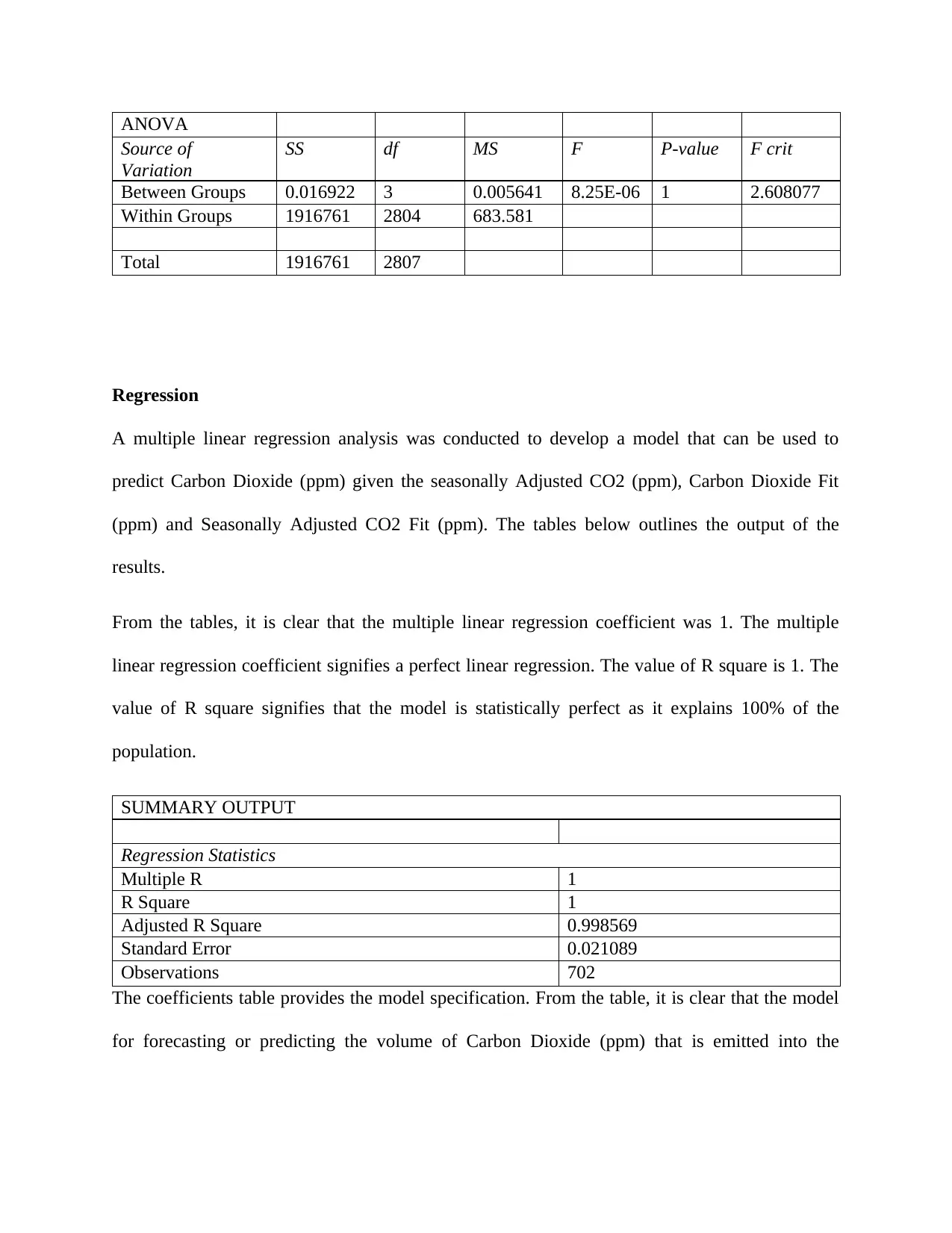
ANOVA
Source of
Variation
SS df MS F P-value F crit
Between Groups 0.016922 3 0.005641 8.25E-06 1 2.608077
Within Groups 1916761 2804 683.581
Total 1916761 2807
Regression
A multiple linear regression analysis was conducted to develop a model that can be used to
predict Carbon Dioxide (ppm) given the seasonally Adjusted CO2 (ppm), Carbon Dioxide Fit
(ppm) and Seasonally Adjusted CO2 Fit (ppm). The tables below outlines the output of the
results.
From the tables, it is clear that the multiple linear regression coefficient was 1. The multiple
linear regression coefficient signifies a perfect linear regression. The value of R square is 1. The
value of R square signifies that the model is statistically perfect as it explains 100% of the
population.
SUMMARY OUTPUT
Regression Statistics
Multiple R 1
R Square 1
Adjusted R Square 0.998569
Standard Error 0.021089
Observations 702
The coefficients table provides the model specification. From the table, it is clear that the model
for forecasting or predicting the volume of Carbon Dioxide (ppm) that is emitted into the
⊘ This is a preview!⊘
Do you want full access?
Subscribe today to unlock all pages.
Trusted by 1+ million students worldwide
1 out of 20
Related Documents


Your All-in-One AI-Powered Toolkit for Academic Success.
+13062052269
info@desklib.com
Available 24*7 on WhatsApp / Email
![[object Object]](/_next/static/media/star-bottom.7253800d.svg)
Unlock your academic potential
Copyright © 2020–2026 A2Z Services. All Rights Reserved. Developed and managed by ZUCOL.