Business Analytics and Statistics Report for Good Harvest (BUS501)
VerifiedAdded on 2020/03/16
|13
|2647
|47
Report
AI Summary
This report presents a business analytics and statistical analysis of sales data for the company Good Harvest, focusing on key performance indicators such as top and worst-selling products, payment method effectiveness, and the impact of product location on sales. The analysis utilizes descriptive statistics, t-tests, and ANOVA to address the CEO's research questions, examining sales performance across different months and seasons. The findings reveal significant differences in sales based on payment methods and product locations, while also identifying top and bottom-performing product categories. Furthermore, the report provides insights into gross profit variations throughout the year and seasonal sales trends. The study aims to provide the CEO with actionable insights to optimize sales strategies and improve overall business performance. The report includes tables summarizing key findings and hypotheses tested, along with a discussion of the results and recommendations for business improvements.
BUS501 - Business Analytics and Statistics
Name:
Lecturer name:
5th October 2017
1
Name:
Lecturer name:
5th October 2017
1
Paraphrase This Document
Need a fresh take? Get an instant paraphrase of this document with our AI Paraphraser
Table of Contents
1. Introduction..............................................................................................................................4
2. Problem definition and business intelligence required.............................................................4
3. Results and findings.................................................................................................................5
Analysis 1: What are the worst and top selling products in terms of sales?................................5
Analysis 2: Is there a difference in payments methods?..............................................................6
Hypothesis 1:............................................................................................................................6
Hypothesis 2:............................................................................................................................7
Analysis 3: How does location of the product in the shop affect the sales performance?...........8
Hypothesis 4:............................................................................................................................8
Analysis 4: How does sakes compare based on the different months of the year?......................8
Hypothesis 5:............................................................................................................................9
How does gross profits compare based on the different months of the year?.............................9
Hypothesis 6:............................................................................................................................9
Analysis 5: How does sales performance compare between different seasons?........................10
Hypothesis 7:..........................................................................................................................10
4. Discussion of the results and recommendations.....................................................................11
References......................................................................................................................................12
2
Table 1: Top selling products..........................................................................................................4
Table 2: Worst selling products.......................................................................................................5
Table 3: t-Test: Two-Sample Assuming Equal Variances..............................................................6
Table 4: t-Test: Two-Sample Assuming Equal Variances..............................................................7
Table 5: Analysis of variance (ANOVA) for the total sales versus product location.....................8
Table 6: Analysis of variance (ANOVA) for the net sales versus months......................................8
Table 7: Analysis of variance (ANOVA) for the gross profits versus months................................9
Table 8: Analysis of variance (ANOVA) for the net sales versus seasons...................................10
3
⊘ This is a preview!⊘
Do you want full access?
Subscribe today to unlock all pages.
Trusted by 1+ million students worldwide
1. Introduction
It is always a desire of each and every organization to maximize on their profits and that is the
key reasons as to why they are in business. This is the case of a young upcoming start up by
the name Good Harvest. The start-up deals in organic farming and as well as sale of their
products direct to their customers. The CEO is concerned about the cost of goods incurred by
the start up as well as the sale performance and revenues generated by the enterprise. Business
analytics can be used to give clear insights on how the enterprise is performing and probably
advise on key areas of improvement. Using the one-year data for the company, we sought to
present the CEO with the key analysis related to key areas mentioned.
2. Problem definition and business intelligence required
Good Harvest has not been to the market for so long; actually they have been barely two
years. The CEO of the company would want to improve the performance of the company but
he has to do it through key data insights gained from analyzing the one year that is available.
However, the CEO has pointed six key research questions he would want to see answered in
the report. His main concern is to understand;
What are the worst and top selling products?
Do payment methods have variation in terms of total cash received?
Do location of the product in the shop have impact on total sales generated?
How do sales performance compare for the different months in a year?
How do profits of the company compare for the different months in a year?
How do sales performance compare for the four seasons?
4
Paraphrase This Document
Need a fresh take? Get an instant paraphrase of this document with our AI Paraphraser
3. Results and findings
Analysis 1: What are the worst and top selling products in terms of sales?
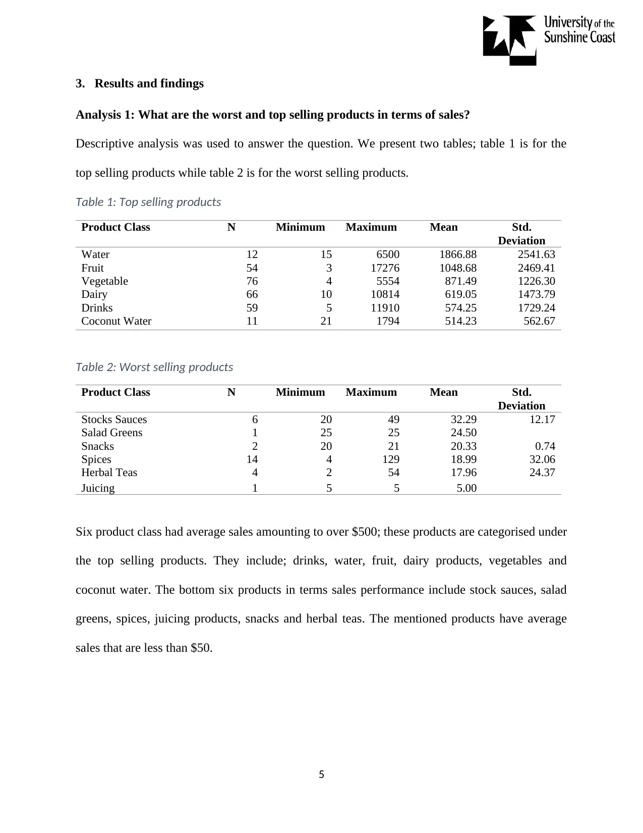
Descriptive analysis was used to answer the question. We present two tables; table 1 is for the
top selling products while table 2 is for the worst selling products.
Table 1: Top selling products
Product Class N Minimum Maximum Mean Std.
Deviation
Water 12 15 6500 1866.88 2541.63
Fruit 54 3 17276 1048.68 2469.41
Vegetable 76 4 5554 871.49 1226.30
Dairy 66 10 10814 619.05 1473.79
Drinks 59 5 11910 574.25 1729.24
Coconut Water 11 21 1794 514.23 562.67
Table 2: Worst selling products
Product Class N Minimum Maximum Mean Std.
Deviation
Stocks Sauces 6 20 49 32.29 12.17
Salad Greens 1 25 25 24.50
Snacks 2 20 21 20.33 0.74
Spices 14 4 129 18.99 32.06
Herbal Teas 4 2 54 17.96 24.37
Juicing 1 5 5 5.00
Six product class had average sales amounting to over $500; these products are categorised under
the top selling products. They include; drinks, water, fruit, dairy products, vegetables and
coconut water. The bottom six products in terms sales performance include stock sauces, salad
greens, spices, juicing products, snacks and herbal teas. The mentioned products have average
sales that are less than $50.
5
Analysis 1: What are the worst and top selling products in terms of sales?
Descriptive analysis was used to answer the question. We present two tables; table 1 is for the
top selling products while table 2 is for the worst selling products.
Table 1: Top selling products
Product Class N Minimum Maximum Mean Std.
Deviation
Water 12 15 6500 1866.88 2541.63
Fruit 54 3 17276 1048.68 2469.41
Vegetable 76 4 5554 871.49 1226.30
Dairy 66 10 10814 619.05 1473.79
Drinks 59 5 11910 574.25 1729.24
Coconut Water 11 21 1794 514.23 562.67
Table 2: Worst selling products
Product Class N Minimum Maximum Mean Std.
Deviation
Stocks Sauces 6 20 49 32.29 12.17
Salad Greens 1 25 25 24.50
Snacks 2 20 21 20.33 0.74
Spices 14 4 129 18.99 32.06
Herbal Teas 4 2 54 17.96 24.37
Juicing 1 5 5 5.00
Six product class had average sales amounting to over $500; these products are categorised under
the top selling products. They include; drinks, water, fruit, dairy products, vegetables and
coconut water. The bottom six products in terms sales performance include stock sauces, salad
greens, spices, juicing products, snacks and herbal teas. The mentioned products have average
sales that are less than $50.
5
Analysis 2: Is there a difference in payments methods?
Organizations do accept different payment methods. There are those which have also restricted
payments from some payment methods. Apparently Good Harvest accepts cash payments, credit
payments, Visa Card payments as well as MasterCard payments. It would be to the interest of the
CEO to understand if there is any of the listed payment methods that brings collects more cash
than the other. That is, the CEO would be interested to know whether there is significant
difference in the total cash received from the four mentioned payment methods. We the four
methods into two categories. One group comprised of cash and credit while the other comprised
of Visa Card and MasterCard. Two hypothesis were then tested.
Hypothesis 1:
H0: There is no significant difference in the total cash received between the cash and the credit
payment methods
H0: There is significant difference in the total cash received between the cash and the credit
payment methods
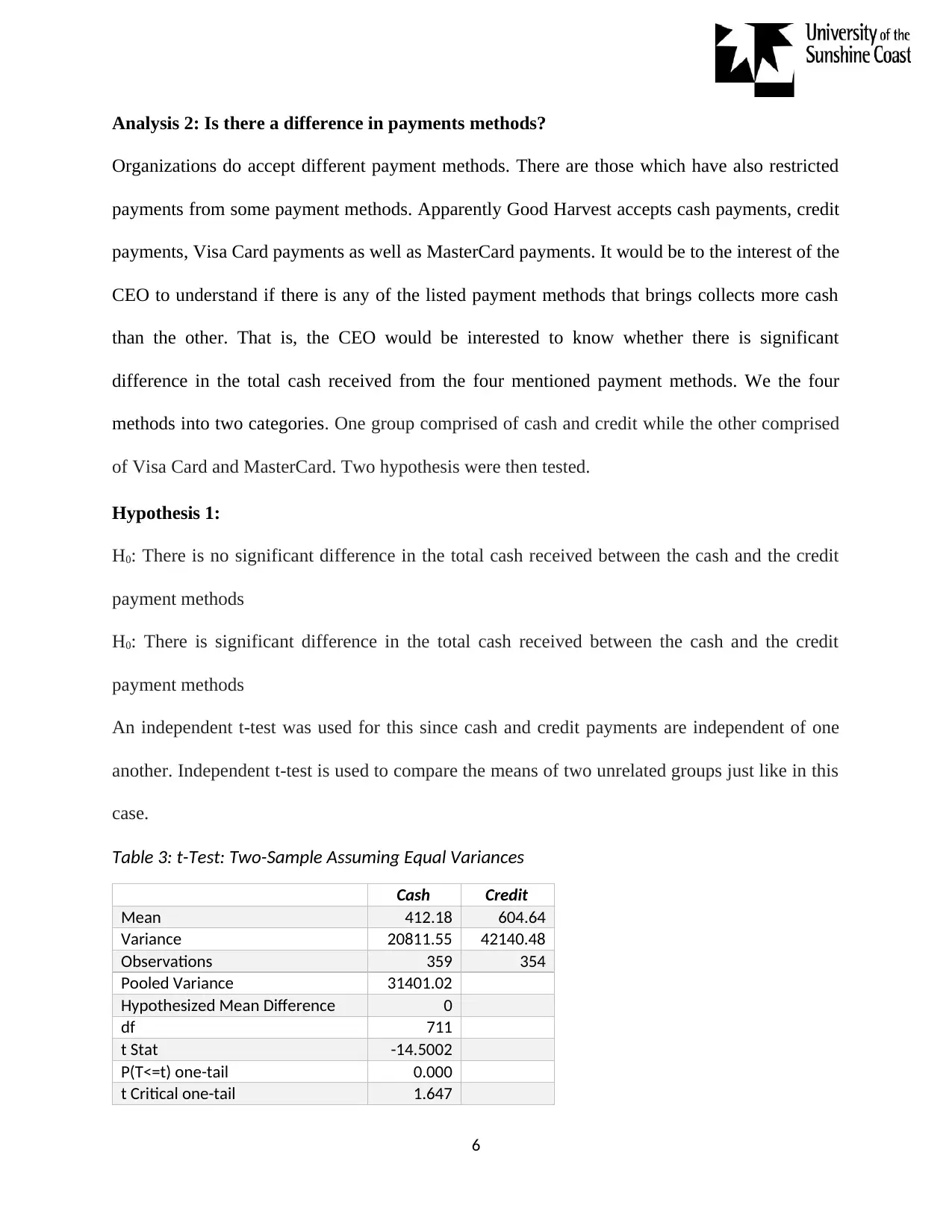
An independent t-test was used for this since cash and credit payments are independent of one
another. Independent t-test is used to compare the means of two unrelated groups just like in this
case.
Table 3: t-Test: Two-Sample Assuming Equal Variances
Cash Credit
Mean 412.18 604.64
Variance 20811.55 42140.48
Observations 359 354
Pooled Variance 31401.02
Hypothesized Mean Difference 0
df 711
t Stat -14.5002
P(T<=t) one-tail 0.000
t Critical one-tail 1.647
6
Organizations do accept different payment methods. There are those which have also restricted
payments from some payment methods. Apparently Good Harvest accepts cash payments, credit
payments, Visa Card payments as well as MasterCard payments. It would be to the interest of the
CEO to understand if there is any of the listed payment methods that brings collects more cash
than the other. That is, the CEO would be interested to know whether there is significant
difference in the total cash received from the four mentioned payment methods. We the four
methods into two categories. One group comprised of cash and credit while the other comprised
of Visa Card and MasterCard. Two hypothesis were then tested.
Hypothesis 1:
H0: There is no significant difference in the total cash received between the cash and the credit
payment methods
H0: There is significant difference in the total cash received between the cash and the credit
payment methods
An independent t-test was used for this since cash and credit payments are independent of one
another. Independent t-test is used to compare the means of two unrelated groups just like in this
case.
Table 3: t-Test: Two-Sample Assuming Equal Variances
Cash Credit
Mean 412.18 604.64
Variance 20811.55 42140.48
Observations 359 354
Pooled Variance 31401.02
Hypothesized Mean Difference 0
df 711
t Stat -14.5002
P(T<=t) one-tail 0.000
t Critical one-tail 1.647
6
⊘ This is a preview!⊘
Do you want full access?
Subscribe today to unlock all pages.
Trusted by 1+ million students worldwide
P(T<=t) two-tail 0.000
t Critical two-tail 1.96
From table 3 above, the p-value was found to be 0.000; this value is less than 5% level of
significance hence we reject the null hypothesis and conclude that there is significant difference
in the total cash received between the cash and the credit payment methods. In fact, it can clearly
be seen that a lot of cash was obtained from the credit payment method as compared to the cash
payment method.
Hypothesis 2:
H0: There is no significant difference in the total cash received between the Visa and the
MasterCard payment methods
H0: There is significant difference in the total cash received between the Visa and the
MasterCard payment methods.
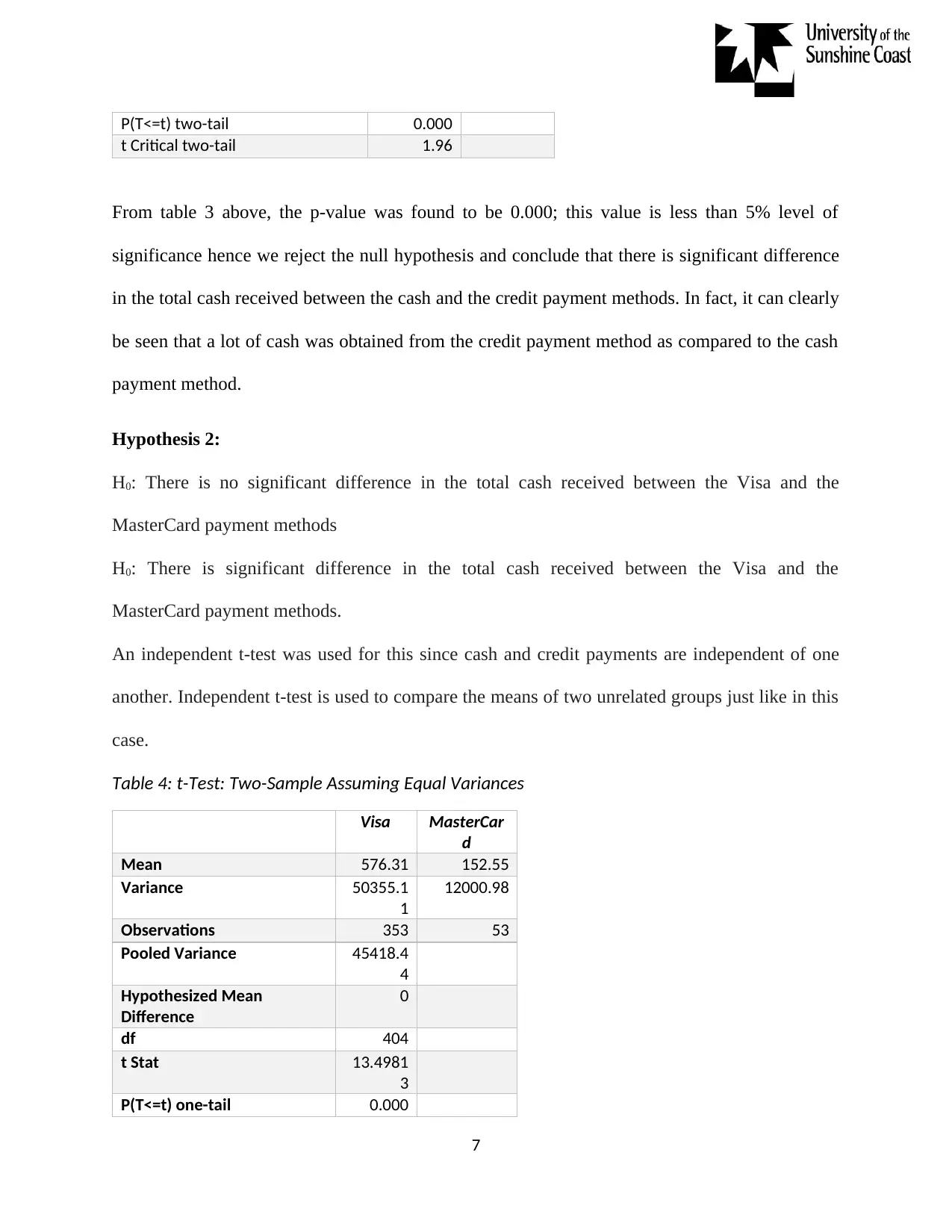
An independent t-test was used for this since cash and credit payments are independent of one
another. Independent t-test is used to compare the means of two unrelated groups just like in this
case.
Table 4: t-Test: Two-Sample Assuming Equal Variances
Visa MasterCar
d
Mean 576.31 152.55
Variance 50355.1
1
12000.98
Observations 353 53
Pooled Variance 45418.4
4
Hypothesized Mean
Difference
0
df 404
t Stat 13.4981
3
P(T<=t) one-tail 0.000
7
t Critical two-tail 1.96
From table 3 above, the p-value was found to be 0.000; this value is less than 5% level of
significance hence we reject the null hypothesis and conclude that there is significant difference
in the total cash received between the cash and the credit payment methods. In fact, it can clearly
be seen that a lot of cash was obtained from the credit payment method as compared to the cash
payment method.
Hypothesis 2:
H0: There is no significant difference in the total cash received between the Visa and the
MasterCard payment methods
H0: There is significant difference in the total cash received between the Visa and the
MasterCard payment methods.
An independent t-test was used for this since cash and credit payments are independent of one
another. Independent t-test is used to compare the means of two unrelated groups just like in this
case.
Table 4: t-Test: Two-Sample Assuming Equal Variances
Visa MasterCar
d
Mean 576.31 152.55
Variance 50355.1
1
12000.98
Observations 353 53
Pooled Variance 45418.4
4
Hypothesized Mean
Difference
0
df 404
t Stat 13.4981
3
P(T<=t) one-tail 0.000
7
Paraphrase This Document
Need a fresh take? Get an instant paraphrase of this document with our AI Paraphraser
t Critical one-tail 1.65
P(T<=t) two-tail 0.000
t Critical two-tail 1.96585
3
From table 4 above, the p-value was found to be 0.000; this value is less than 5% level of
significance hence we reject the null hypothesis and conclude that there is significant difference
in the total cash received from MasterCard and that received from the Visa Card. In fact, it can
clearly be seen that a lot of cash was obtained from the credit payment method as compared to
the cash payment method.
Analysis 3: How does location of the product in the shop affect the sales performance?
The hypothesis tested for this question is given below;
Hypothesis 4:
H0: There is no significant difference in the mean total sales between the different product
locations in the shop
H0: There is significant difference in the mean total sales between the different product locations
in the shop.
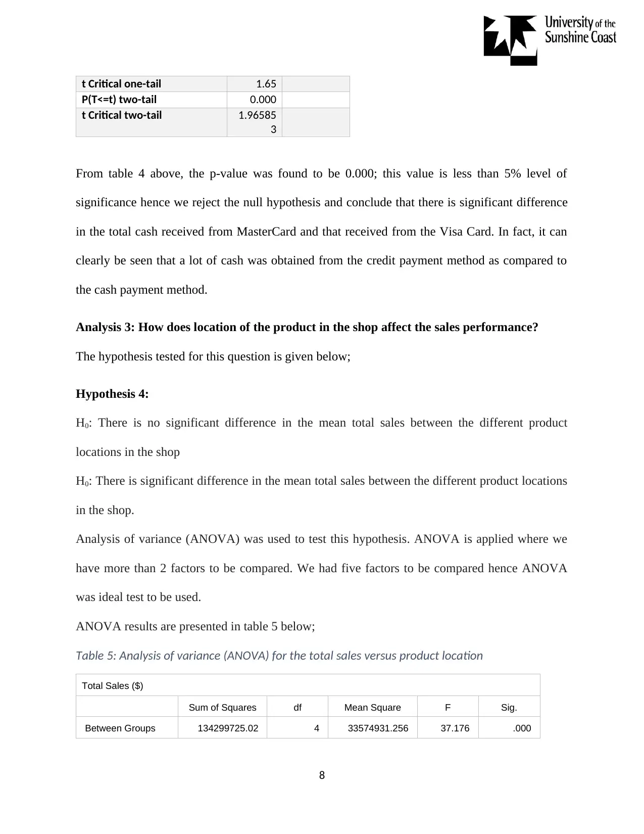
Analysis of variance (ANOVA) was used to test this hypothesis. ANOVA is applied where we
have more than 2 factors to be compared. We had five factors to be compared hence ANOVA
was ideal test to be used.
ANOVA results are presented in table 5 below;
Table 5: Analysis of variance (ANOVA) for the total sales versus product location
Total Sales ($)
Sum of Squares df Mean Square F Sig.
Between Groups 134299725.02 4 33574931.256 37.176 .000
8
P(T<=t) two-tail 0.000
t Critical two-tail 1.96585
3
From table 4 above, the p-value was found to be 0.000; this value is less than 5% level of
significance hence we reject the null hypothesis and conclude that there is significant difference
in the total cash received from MasterCard and that received from the Visa Card. In fact, it can
clearly be seen that a lot of cash was obtained from the credit payment method as compared to
the cash payment method.
Analysis 3: How does location of the product in the shop affect the sales performance?
The hypothesis tested for this question is given below;
Hypothesis 4:
H0: There is no significant difference in the mean total sales between the different product
locations in the shop
H0: There is significant difference in the mean total sales between the different product locations
in the shop.
Analysis of variance (ANOVA) was used to test this hypothesis. ANOVA is applied where we
have more than 2 factors to be compared. We had five factors to be compared hence ANOVA
was ideal test to be used.
ANOVA results are presented in table 5 below;
Table 5: Analysis of variance (ANOVA) for the total sales versus product location
Total Sales ($)
Sum of Squares df Mean Square F Sig.
Between Groups 134299725.02 4 33574931.256 37.176 .000
8
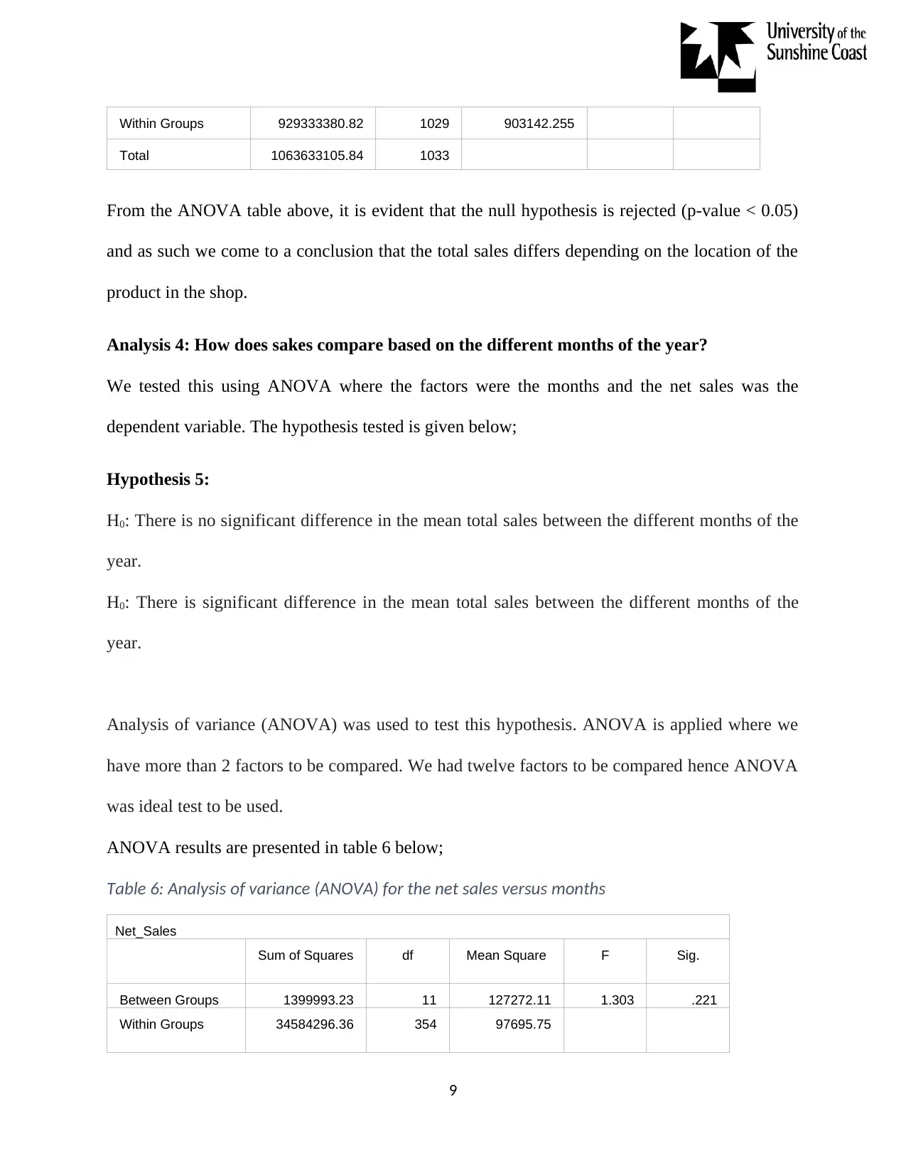
Within Groups 929333380.82 1029 903142.255
Total 1063633105.84 1033
From the ANOVA table above, it is evident that the null hypothesis is rejected (p-value < 0.05)
and as such we come to a conclusion that the total sales differs depending on the location of the
product in the shop.
Analysis 4: How does sakes compare based on the different months of the year?
We tested this using ANOVA where the factors were the months and the net sales was the
dependent variable. The hypothesis tested is given below;
Hypothesis 5:
H0: There is no significant difference in the mean total sales between the different months of the
year.
H0: There is significant difference in the mean total sales between the different months of the
year.
Analysis of variance (ANOVA) was used to test this hypothesis. ANOVA is applied where we
have more than 2 factors to be compared. We had twelve factors to be compared hence ANOVA
was ideal test to be used.
ANOVA results are presented in table 6 below;
Table 6: Analysis of variance (ANOVA) for the net sales versus months
Net_Sales
Sum of Squares df Mean Square F Sig.
Between Groups 1399993.23 11 127272.11 1.303 .221
Within Groups 34584296.36 354 97695.75
9
⊘ This is a preview!⊘
Do you want full access?
Subscribe today to unlock all pages.
Trusted by 1+ million students worldwide
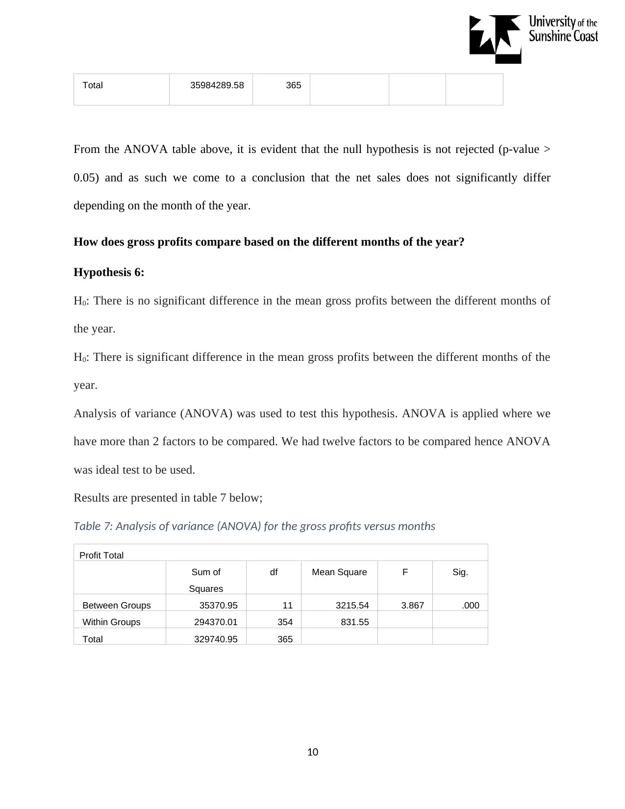
Total 35984289.58 365
From the ANOVA table above, it is evident that the null hypothesis is not rejected (p-value >
0.05) and as such we come to a conclusion that the net sales does not significantly differ
depending on the month of the year.
How does gross profits compare based on the different months of the year?
Hypothesis 6:
H0: There is no significant difference in the mean gross profits between the different months of
the year.
H0: There is significant difference in the mean gross profits between the different months of the
year.
Analysis of variance (ANOVA) was used to test this hypothesis. ANOVA is applied where we
have more than 2 factors to be compared. We had twelve factors to be compared hence ANOVA
was ideal test to be used.
Results are presented in table 7 below;
Table 7: Analysis of variance (ANOVA) for the gross profits versus months
Profit Total
Sum of
Squares
df Mean Square F Sig.
Between Groups 35370.95 11 3215.54 3.867 .000
Within Groups 294370.01 354 831.55
Total 329740.95 365
10
Paraphrase This Document
Need a fresh take? Get an instant paraphrase of this document with our AI Paraphraser
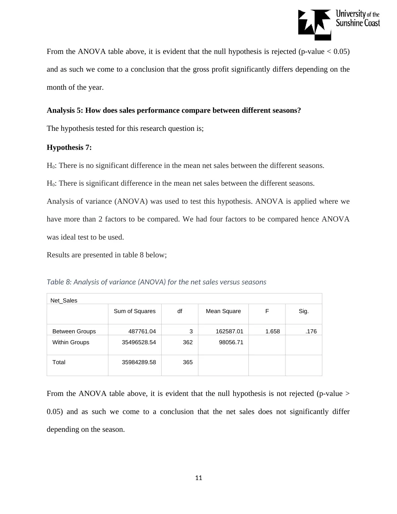
From the ANOVA table above, it is evident that the null hypothesis is rejected (p-value < 0.05)
and as such we come to a conclusion that the gross profit significantly differs depending on the
month of the year.
Analysis 5: How does sales performance compare between different seasons?
The hypothesis tested for this research question is;
Hypothesis 7:
H0: There is no significant difference in the mean net sales between the different seasons.
H0: There is significant difference in the mean net sales between the different seasons.
Analysis of variance (ANOVA) was used to test this hypothesis. ANOVA is applied where we
have more than 2 factors to be compared. We had four factors to be compared hence ANOVA
was ideal test to be used.
Results are presented in table 8 below;
Table 8: Analysis of variance (ANOVA) for the net sales versus seasons
Net_Sales
Sum of Squares df Mean Square F Sig.
Between Groups 487761.04 3 162587.01 1.658 .176
Within Groups 35496528.54 362 98056.71
Total 35984289.58 365
From the ANOVA table above, it is evident that the null hypothesis is not rejected (p-value >
0.05) and as such we come to a conclusion that the net sales does not significantly differ
depending on the season.
11
4. Discussion of the results and recommendations
Interesting findings came out of this study. First we were able to identify both the top performing
products as well as the worst performing products. Some of the top performing products were
drinks, water, vegetables, dairy products, fruits among others while the main products that were
identified to perform poorly included; stock sauces, salad greens, spices, juicing products, snacks
and herbal teas. Results showed that month of the year had no influence on the net sales of the
company however it had significant influence on the gross profits of the company. Seasons also
didn’t have significant influence on the net sales. Location of the product in the shop had
significant effect on the sales performance of the company.
Based on the listed findings, it is evident that cost of goods varies depending on the month of the
year hence affecting the gross profits of the company. It would therefore be advisable for the
CEO of the Good harvest company to try understanding how the cost of goods compare within
the different months. For instance, are the labour costs high in some months? Are the cost of
materials higher in some months? Answering these questions will help the CEO to plan when to
hire workers and when to make purchases of the materials to avoid doing it when the costs are
high. By this the company will be able to maximize on its profit while minimizing of the
expenditure costs.
The CEO should also put much emphasis on ensuring that the display of the products is looked at
in a more appropriate manner. Results showed that sales performance of the products varied
depending on where the product was located in the shop.
12
⊘ This is a preview!⊘
Do you want full access?
Subscribe today to unlock all pages.
Trusted by 1+ million students worldwide
1 out of 13
Related Documents


Your All-in-One AI-Powered Toolkit for Academic Success.
+13062052269
info@desklib.com
Available 24*7 on WhatsApp / Email
![[object Object]](/_next/static/media/star-bottom.7253800d.svg)
Unlock your academic potential
Copyright © 2020–2026 A2Z Services. All Rights Reserved. Developed and managed by ZUCOL.