Good Harvest Business Analytics & Statistics Research Report: BUS 501
VerifiedAdded on 2020/03/16
|12
|2264
|103
Report
AI Summary
This research report analyzes the sales data of Good Harvest, a health food shop. The report examines two datasets encompassing sales information for the company's first year. The study addresses four key research questions: identifying top/worst-selling products, analyzing payment method differences, assessing sales performance based on product location, and evaluating sales and gross profit variations across different months and seasons. The methodology includes descriptive statistics, ANOVA tests, and chi-square tests. Key findings reveal that vegetables are the best-selling products, while juicing is the worst. The report concludes that product location significantly impacts sales, and there are no significant differences in sales between months or seasons. Recommendations include focusing on vegetable stock and strategic product placement to enhance sales and revenue. The report provides detailed tables and statistical analysis to support these conclusions, offering valuable insights into Good Harvest's business operations and performance.
Research Report
Name:
Student Number:
Tutor:
BUS 501
Business Analytics & Statistics
5th October 2017
1
Name:
Student Number:
Tutor:
BUS 501
Business Analytics & Statistics
5th October 2017
1
Paraphrase This Document
Need a fresh take? Get an instant paraphrase of this document with our AI Paraphraser
Table of content
Introduction......................................................................................................................................2
Problem definition and business intelligence..................................................................................2
Visualization and descriptive statistics............................................................................................4
Results and Analysis........................................................................................................................6
Discussion and recommendations..................................................................................................10
References......................................................................................................................................10
2
Introduction
Good harvest is a small health food shop in Sunshine coast which sales organic food and has
been in operation for a year now and it moving to the second year in business (Harvest, n.d.).
They deliver weekly organic produce directly from their farms and other local farms directly the
customers’ doorstep using their home delivery service model. Good harvest farm produce ranges
from Ayurvedic, bakery, dairy, drinks, fruit, grocery, harvest kitchen etc. up to water. Their main
mission is to connect local community or local people with local farmers, supplying chemical
free and safe produce at an affordable price, support farmers who invest in ecologically
responsible farming and finally provide education on seasonal, nutrition consumption and
sustainability. However, there are problems affecting this agribusiness industry as stated by
(Lowe, 2004) that the supply of food in agribusiness is characterized by a number of
uncertainties in both supply and demand chain and it required better technological tools and
management in decision making in the sector. Good harvest is facing challenges of high cost of
goods to be sold to the customers, revenue which might be lower depending on the sales and
finally average sales. Good harvest might also face problems of people in the community
wanting to buy produce which are not local and also the problem of supply and demand where
the local farmers aren’t able to meet demand with their supply.
Problem definition and business intelligence
Two datasets were provided which had data for sales from Good Harvest Company on all their
sales for their first year in business. Our data variables for the first dataset were product class,
product name, product category, quantity, weight, total sales, COGS, net profit, location in the
shop and total profit. For the second data set our variables were day, month, season, GST
inclusive, GST exclusive, gross sales, net sales, total cash, credit total, MasterCard total, visa
3
⊘ This is a preview!⊘
Do you want full access?
Subscribe today to unlock all pages.
Trusted by 1+ million students worldwide
total, house account, total orders, average sales, staff cost, weekday, rainfall and profit total. We
had four research questions as listed below
1. What are the top/worst selling products in terms of sales?
a. Is there a difference in payment methods?
2. Are the differences in sales performance based on where the product is located in the
shop? How does this effect both profits and revenue?
3. Is there a difference in sales and gross profit between different months of the year?
4. Are their differences in sales performance between different seasons?
a. How does this relate to rainfall and profit?
A number of statistical methodologies were applied to answer the above research question
which ranged from test of association (chi-square test of association), test of difference of means
(t test methods) (Rouder, 2009) descriptive statistics using custom tables. For the first research
question (1) SPSS custom tables was used to produce the results where products were placed in
the row field and sum of sales on the column field the reason for using this method is to produce
results which are tabulated for easy comparison among the produce. The second part of the
question (1.a) which was used to test if there was a difference is payment method, a one way
ANOVA was applied to test the significance since one way ANOVA tests whether the mean
value of all payment methods was equal. On the second research question, we tested the
association between sales and location of the product in the shop using chi-square test of
association the reason is that chi-square help us to find out whether there is an association
between the variables (Goodman, 1971). On the second part of the question custom tables were
used to show the distribution of sales and profit against location in the shop the reason is for
provision of good visualization to help in comparison. On the third question one way ANOVA
4
Paraphrase This Document
Need a fresh take? Get an instant paraphrase of this document with our AI Paraphraser
was used for comparison of means of profit and sales within months. Finally, on the last
question, one way ANOVA was used to test the whether the mean sales within seasons were
different and on the second part of the question custom tables was used to show the distribution.
Visualization and descriptive statistics
Descriptive statistics are simple statistics which describe variables, this include mean, range,
variance etc. (Daniel, 1995).
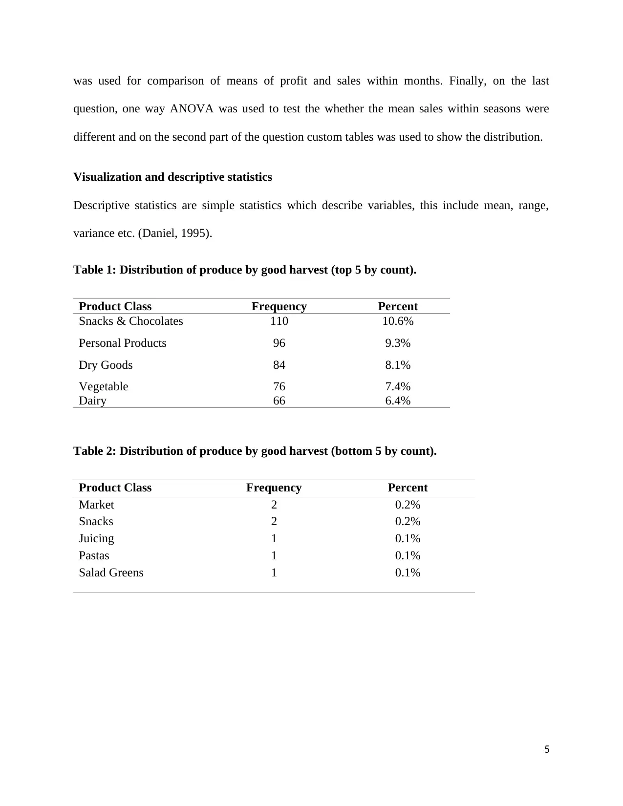
Table 1: Distribution of produce by good harvest (top 5 by count).
Product Class Frequency Percent
Snacks & Chocolates 110 10.6%
Personal Products 96 9.3%
Dry Goods 84 8.1%
Vegetable 76 7.4%
Dairy 66 6.4%
Table 2: Distribution of produce by good harvest (bottom 5 by count).
Product Class Frequency Percent
Market 2 0.2%
Snacks 2 0.2%
Juicing 1 0.1%
Pastas 1 0.1%
Salad Greens 1 0.1%
5
question, one way ANOVA was used to test the whether the mean sales within seasons were
different and on the second part of the question custom tables was used to show the distribution.
Visualization and descriptive statistics
Descriptive statistics are simple statistics which describe variables, this include mean, range,
variance etc. (Daniel, 1995).
Table 1: Distribution of produce by good harvest (top 5 by count).
Product Class Frequency Percent
Snacks & Chocolates 110 10.6%
Personal Products 96 9.3%
Dry Goods 84 8.1%
Vegetable 76 7.4%
Dairy 66 6.4%
Table 2: Distribution of produce by good harvest (bottom 5 by count).
Product Class Frequency Percent
Market 2 0.2%
Snacks 2 0.2%
Juicing 1 0.1%
Pastas 1 0.1%
Salad Greens 1 0.1%
5
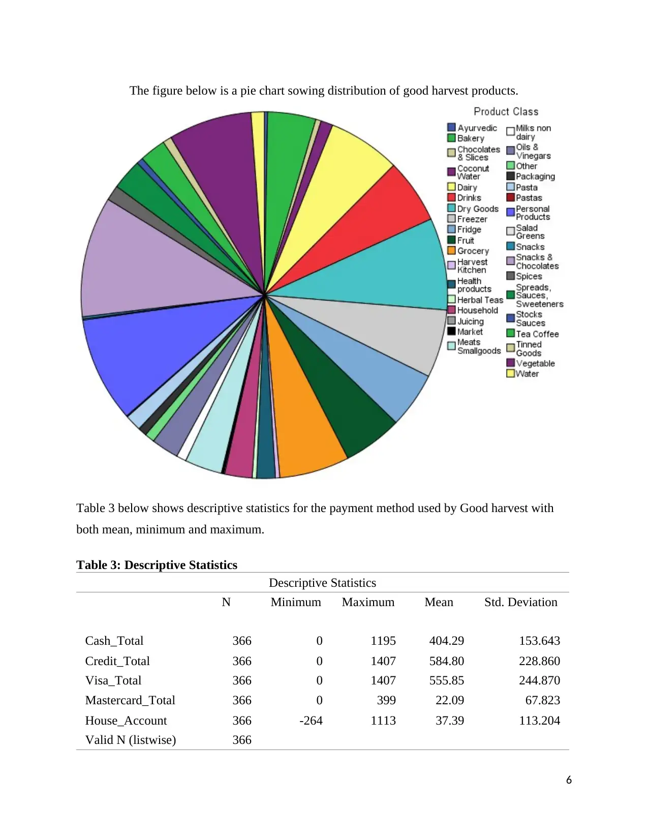
The figure below is a pie chart sowing distribution of good harvest products.
Table 3 below shows descriptive statistics for the payment method used by Good harvest with
both mean, minimum and maximum.
Table 3: Descriptive Statistics
Descriptive Statistics
N Minimum Maximum Mean Std. Deviation
Cash_Total 366 0 1195 404.29 153.643
Credit_Total 366 0 1407 584.80 228.860
Visa_Total 366 0 1407 555.85 244.870
Mastercard_Total 366 0 399 22.09 67.823
House_Account 366 -264 1113 37.39 113.204
Valid N (listwise) 366
6
⊘ This is a preview!⊘
Do you want full access?
Subscribe today to unlock all pages.
Trusted by 1+ million students worldwide
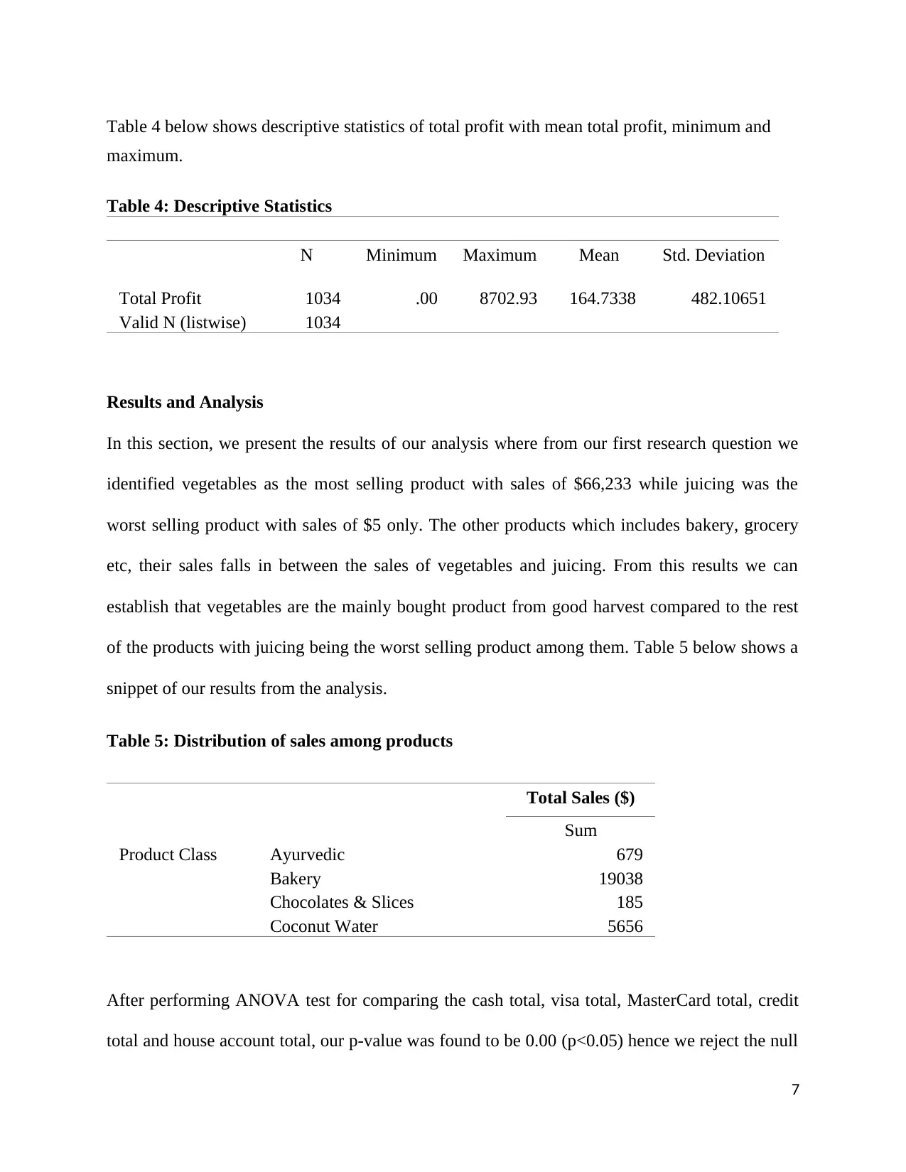
Table 4 below shows descriptive statistics of total profit with mean total profit, minimum and
maximum.
Table 4: Descriptive Statistics
N Minimum Maximum Mean Std. Deviation
Total Profit 1034 .00 8702.93 164.7338 482.10651
Valid N (listwise) 1034
Results and Analysis
In this section, we present the results of our analysis where from our first research question we
identified vegetables as the most selling product with sales of $66,233 while juicing was the
worst selling product with sales of $5 only. The other products which includes bakery, grocery
etc, their sales falls in between the sales of vegetables and juicing. From this results we can
establish that vegetables are the mainly bought product from good harvest compared to the rest
of the products with juicing being the worst selling product among them. Table 5 below shows a
snippet of our results from the analysis.
Table 5: Distribution of sales among products
Total Sales ($)
Sum
Product Class Ayurvedic 679
Bakery 19038
Chocolates & Slices 185
Coconut Water 5656
After performing ANOVA test for comparing the cash total, visa total, MasterCard total, credit
total and house account total, our p-value was found to be 0.00 (p<0.05) hence we reject the null
7
Paraphrase This Document
Need a fresh take? Get an instant paraphrase of this document with our AI Paraphraser
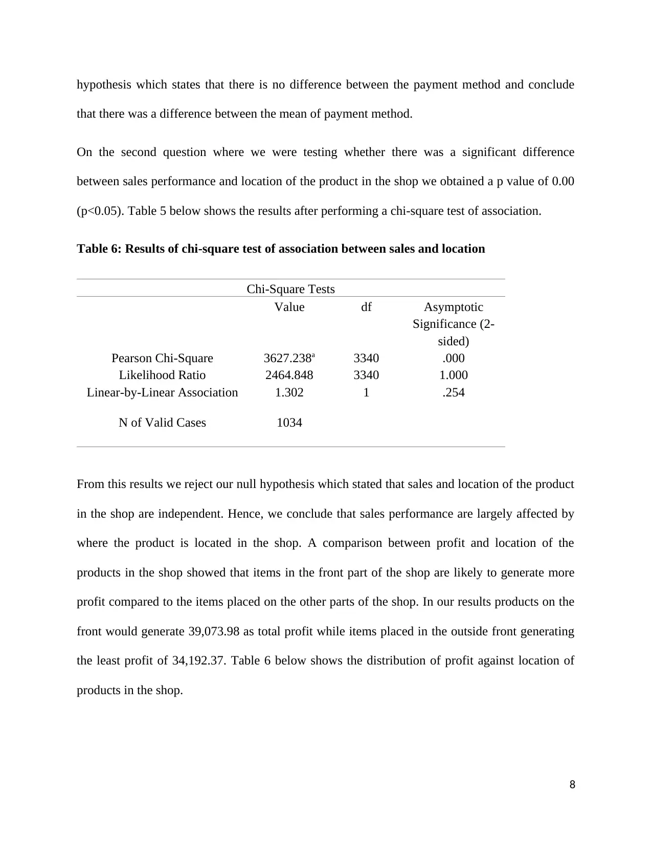
hypothesis which states that there is no difference between the payment method and conclude
that there was a difference between the mean of payment method.
On the second question where we were testing whether there was a significant difference
between sales performance and location of the product in the shop we obtained a p value of 0.00
(p<0.05). Table 5 below shows the results after performing a chi-square test of association.
Table 6: Results of chi-square test of association between sales and location
Chi-Square Tests
Value df Asymptotic
Significance (2-
sided)
Pearson Chi-Square 3627.238a 3340 .000
Likelihood Ratio 2464.848 3340 1.000
Linear-by-Linear Association 1.302 1 .254
N of Valid Cases 1034
From this results we reject our null hypothesis which stated that sales and location of the product
in the shop are independent. Hence, we conclude that sales performance are largely affected by
where the product is located in the shop. A comparison between profit and location of the
products in the shop showed that items in the front part of the shop are likely to generate more
profit compared to the items placed on the other parts of the shop. In our results products on the
front would generate 39,073.98 as total profit while items placed in the outside front generating
the least profit of 34,192.37. Table 6 below shows the distribution of profit against location of
products in the shop.
8
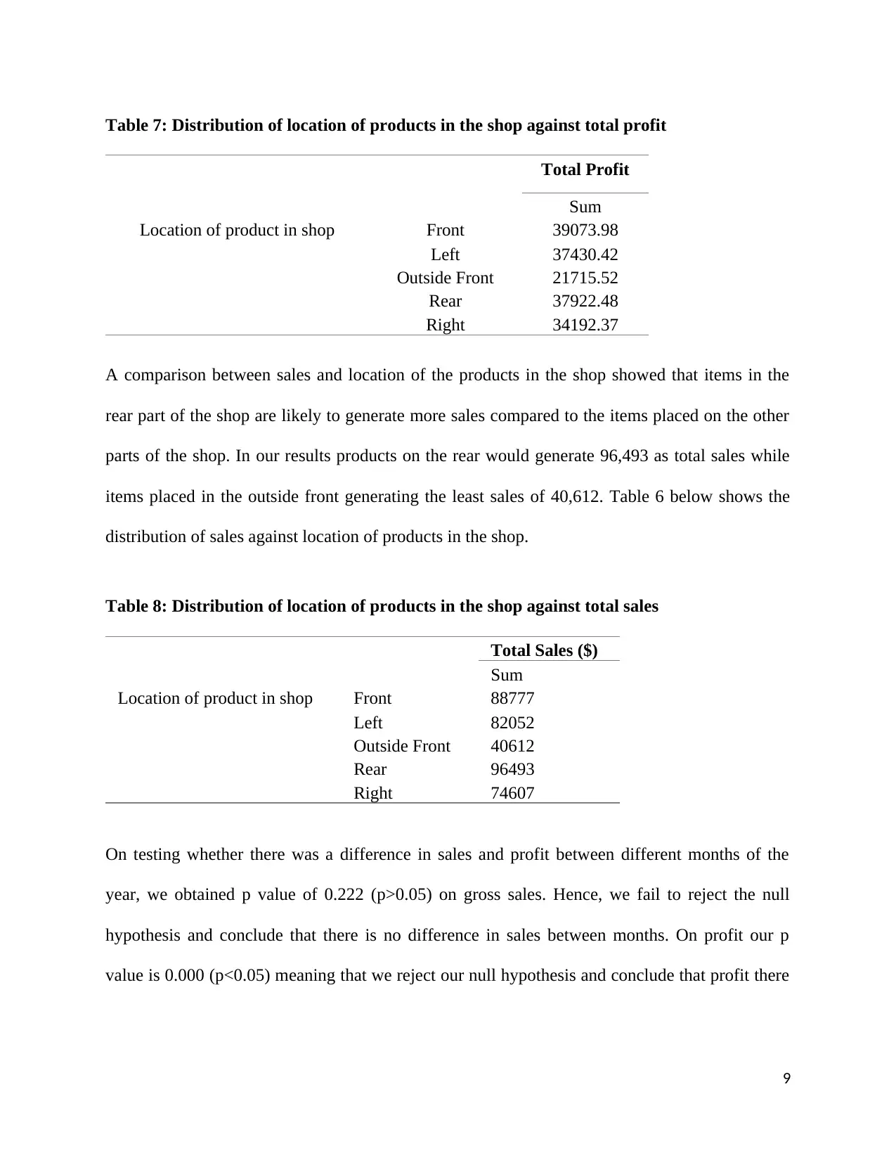
Table 7: Distribution of location of products in the shop against total profit
Total Profit
Sum
Location of product in shop Front 39073.98
Left 37430.42
Outside Front 21715.52
Rear 37922.48
Right 34192.37
A comparison between sales and location of the products in the shop showed that items in the
rear part of the shop are likely to generate more sales compared to the items placed on the other
parts of the shop. In our results products on the rear would generate 96,493 as total sales while
items placed in the outside front generating the least sales of 40,612. Table 6 below shows the
distribution of sales against location of products in the shop.
Table 8: Distribution of location of products in the shop against total sales
Total Sales ($)
Sum
Location of product in shop Front 88777
Left 82052
Outside Front 40612
Rear 96493
Right 74607
On testing whether there was a difference in sales and profit between different months of the
year, we obtained p value of 0.222 (p>0.05) on gross sales. Hence, we fail to reject the null
hypothesis and conclude that there is no difference in sales between months. On profit our p
value is 0.000 (p<0.05) meaning that we reject our null hypothesis and conclude that profit there
9
⊘ This is a preview!⊘
Do you want full access?
Subscribe today to unlock all pages.
Trusted by 1+ million students worldwide
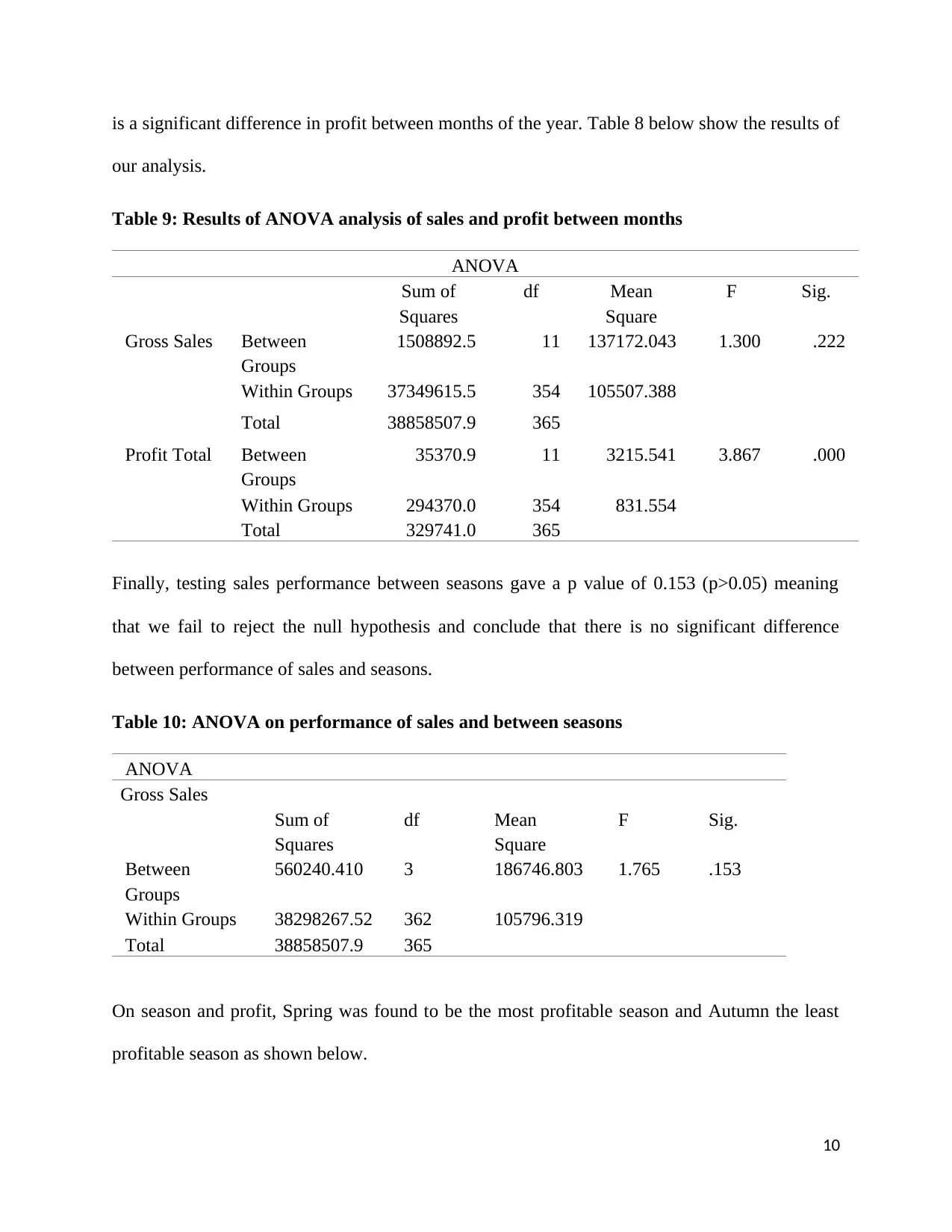
is a significant difference in profit between months of the year. Table 8 below show the results of
our analysis.
Table 9: Results of ANOVA analysis of sales and profit between months
ANOVA
Sum of
Squares
df Mean
Square
F Sig.
Gross Sales Between
Groups
1508892.5 11 137172.043 1.300 .222
Within Groups 37349615.5 354 105507.388
Total 38858507.9 365
Profit Total Between
Groups
35370.9 11 3215.541 3.867 .000
Within Groups 294370.0 354 831.554
Total 329741.0 365
Finally, testing sales performance between seasons gave a p value of 0.153 (p>0.05) meaning
that we fail to reject the null hypothesis and conclude that there is no significant difference
between performance of sales and seasons.
Table 10: ANOVA on performance of sales and between seasons
ANOVA
Gross Sales
Sum of
Squares
df Mean
Square
F Sig.
Between
Groups
560240.410 3 186746.803 1.765 .153
Within Groups 38298267.52 362 105796.319
Total 38858507.9 365
On season and profit, Spring was found to be the most profitable season and Autumn the least
profitable season as shown below.
10
Paraphrase This Document
Need a fresh take? Get an instant paraphrase of this document with our AI Paraphraser
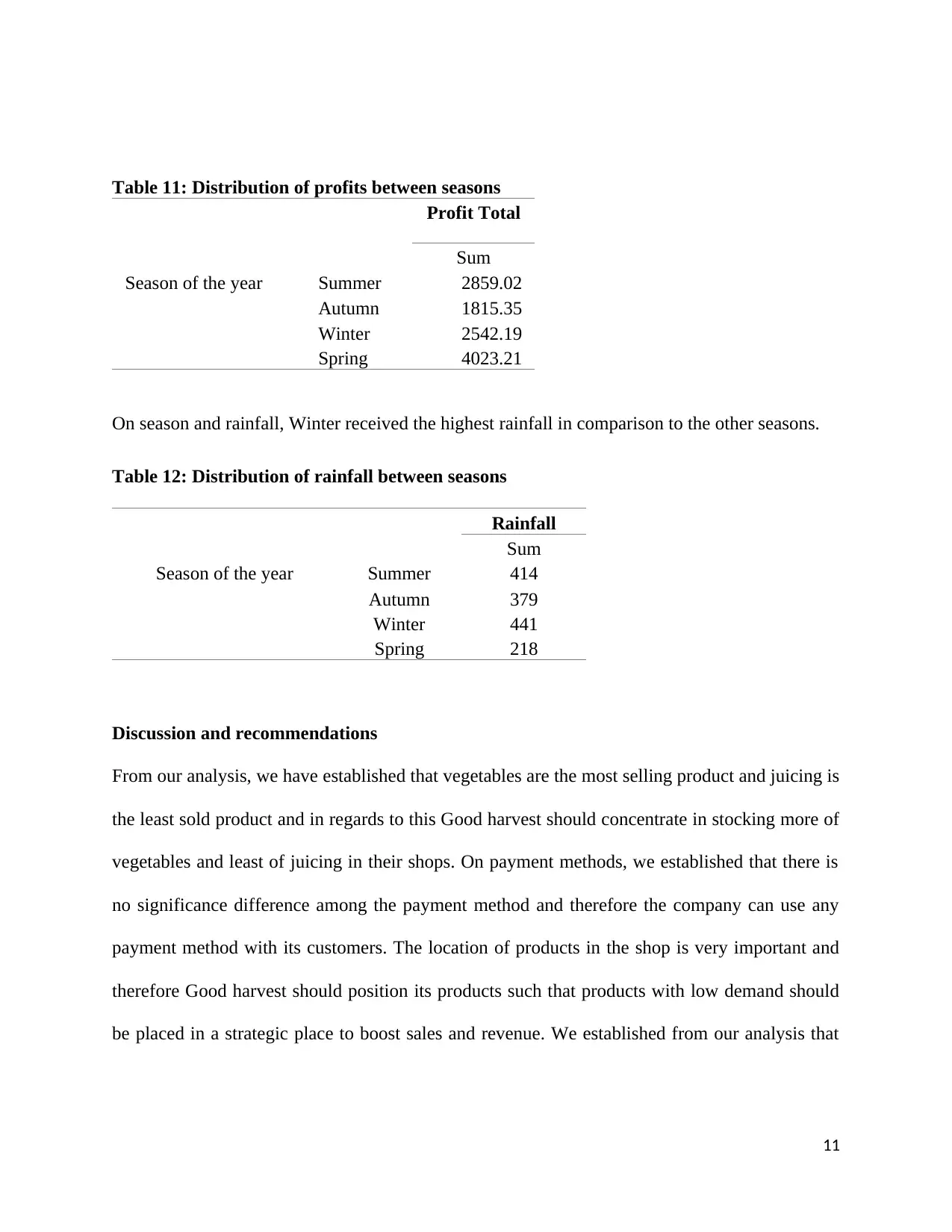
Table 11: Distribution of profits between seasons
Profit Total
Sum
Season of the year Summer 2859.02
Autumn 1815.35
Winter 2542.19
Spring 4023.21
On season and rainfall, Winter received the highest rainfall in comparison to the other seasons.
Table 12: Distribution of rainfall between seasons
Rainfall
Sum
Season of the year Summer 414
Autumn 379
Winter 441
Spring 218
Discussion and recommendations
From our analysis, we have established that vegetables are the most selling product and juicing is
the least sold product and in regards to this Good harvest should concentrate in stocking more of
vegetables and least of juicing in their shops. On payment methods, we established that there is
no significance difference among the payment method and therefore the company can use any
payment method with its customers. The location of products in the shop is very important and
therefore Good harvest should position its products such that products with low demand should
be placed in a strategic place to boost sales and revenue. We established from our analysis that
11
there is no significant difference in sales between months and season and this means that the
company can always make sales regardless of the month or the season of the year.
References
Anova, S., 2002. Statistical computing: an introduction to data analysis using S-Plus.
Daniel, W., 1995. Biostatistics: a foundation for analysis in the health sciences..
Goodman, L., 1971. Partitioning of chi-square, analysis of marginal contingency tables, and
estimation of expected frequencies in multidimensional contingency tables. Journal of the
American statistical Association, pp. 66(334), pp.339-344.
Harvest, G., n.d. good harvest organic. [Online]
Available at: goodharvest.com.au
Lowe, T., 2004. Decision technologies for agribusiness problems: A brief review of selected
literature and a call for research. Manufacturing & Service Operations Management, 6(3),
pp.201-208.6(3). s.l.:s.n.
Rouder, J., 2009. Bayesian t tests for accepting and rejecting the null hypothesis. .
12
⊘ This is a preview!⊘
Do you want full access?
Subscribe today to unlock all pages.
Trusted by 1+ million students worldwide
1 out of 12
Related Documents


Your All-in-One AI-Powered Toolkit for Academic Success.
+13062052269
info@desklib.com
Available 24*7 on WhatsApp / Email
![[object Object]](/_next/static/media/star-bottom.7253800d.svg)
Unlock your academic potential
Copyright © 2020–2026 A2Z Services. All Rights Reserved. Developed and managed by ZUCOL.