The Gravity Model and Trade Efficiency: A Stochastic Frontier Analysis

This paper investigates trade efficiency among Eastern and Western European countries using a stochastic frontier analysis of the gravity model. It examines bilateral exports from 17 Western European countries to 10 new member states between 1994 and 2007, a period marked by significant economic transformation. The study constructs a trade frontier representing the maximum possible level of bilateral trade and generates efficiency scores to assess the degree of East-West trade integration. The findings suggest a high degree of trade integration, with new member states achieving approximately two-thirds of their frontier estimates, indicating low trade resistances. The research highlights exceptions to this pattern, identifying countries with the greatest potential for trade expansion. The analysis contributes to the literature by evaluating trade performance against a maximum potential level defined by a stochastic frontier, offering insights into trade dynamics and potential areas for growth.

DISCUSSION PAPERS
IN
ECONOMICS
No. 2013/4 ISSN 1478-9396
THE GRAVITY MODEL AND TRADE
EFFICIENCY: A STOCHASTIC FRONTIER
ANALYSIS OF POTENTIAL TRADE
GEETHA RAVISHANKAR

DISCUSSION PAPERS IN ECONOMICS
The economic research undertaken at Nottingham Trent University
covers various fields of economics. But, a large part of it was grouped
into two categories, Applied Economics and Policy and Political
Economy.
This paper is part of the new series, Discussion Papers in
Economics.
Earlier papers in all series can be found at:
http://www.ntu.ac.uk/research/research_at_ntu/academic_schools/nbs
/working_papers.html
Enquiries concerning this or any of our other Discussion Papers should
be addressed to the Editors:
Dr. Marie Stack, Email: [e-mail]
Dr. Dan Wheatley, Email: [e-mail]
Division of Economics
Nottingham Trent University
Burton Street, Nottingham, NG1 4BU
UNITED KINGDOM.

The Gravity Model and Trade Efficiency:
A Stochastic Frontier Analysis of Potential Trade
ABSTRACT
The opening up process of the eastern European countries is characterised by an
increasing degree of trade integration with their Western neigbouring countries.
Typically, the degree of East West trade integration is assessed by comparing actual trade
volumes with potential trade volumes projected from the gravity model parameters
estimated for a group of countries that best represent normal trade relations. This
approach, however, does not compare trade levels against a maximum level of trade
feasible for the group of eastern European countries. This paper by using a stochastic
frontier specification of the gravity model is able to identify the efficiency of trade
integration relative to maximum potential levels. The findings, based on a panel data set
of bilateral exports from 17 Western European countries to the 10 new member states
over the 1994 2007 period, indicate a high degree of East West trade integration close to
two thirds of frontier estimates, suggesting a low degree of trade resistances.
JEL Classification: C33, F14, F15
Keywords: Gravity model, Potential trade, Efficiency scores

1. INTRODUCTION
Not unlike the drive to increase trade between the established European Union (EU)
member countries as part of a customs union, the opening up process of the eastern
European countries began with trade integration. Strong bilateral trade links were formed
in advance of formal EU entry. After the Council for Mutual Economic Assistance
(CMEA) system1 was dissolved in the early 1990s, a new era of trade expansion was
ushered in, culminating in the Western European countries becoming the main trading
partners for the excommunist countries.
Figure 1 plots each new EU member country’s share of world trade (exports plus
imports) with the Western European countries. By 1994, Western Europe had already
become important trading partners for the group of ten, implying an almost immediate
release of economic ties from the former Soviet Union. Trailing behind its counterparts,
Lithuania was initially the slowest to open up its trade links, but increased its trade shares
by 1.5 times within a decade. Slovakia experienced an even more dramatic reorientation
of trade westwards, rising by two thirds to its peak levels in 2003. Conducting about half
of its trade with the Western countries in 1993, the trade shares for Bulgaria and Romania
depict an almost parallel trend, but with the latter maintaining a ten per cent lead over the
former. Much like Bulgaria’s path, the trade shares for Estonia and Latvia have ended up
like they started albeit with some variation in between. The trade shares for the top four
ranking countries, namely the Czech Republic, Hungary, Poland and Slovenia remain

A two stage gravity approach to projecting East West trade volumes is the usual
route to assessing bilateral trade performance. In the first stage, the gravity model of trade
is estimated for a group of countries that best represent normal trade relations. In its basic
form, the standard gravity equation explains bilateral trade as a function of the economic
size of two countries and the distance between them (Tinbergen 1962; Pöyhönen 1963).
The augmented version additionally includes income per head for both countries and
other trade impeding or trade stimulating factors (Bergstrand 1989).
In the second stage, the gravity model parameters that fit a model of a normal
country’s geographic trade patterns are used to project the expected trade flows in an East
West direction. The trade flows predicted by the model can then be compared with actual
trade flows to assess the likelihood for future expansion or depletion of trade links
between a pair of countries. Whereas a value in excess of unity suggests remaining
potential for trade growth, a value of less than unity suggests trade potential is already
exhausted. In this way, the potential to actual trade ratios are informative as to the degree
of East West trade integration under normal conditions.
The two stage approach to trade projections pervades the empirical literature (see,
for example, Baldwin 1994; Gros and Gonciarz 1996; Stack and Pentecost 2010). In
assuming full economic liberalisation, these studies define East West potential trade in
terms of the sample average, usually the Western European countries. In other words, the
mean effects of trade determinants are estimated, implying potential trade is assessed

trade performance against a maximum possible level of potential trade defined by a
stochastic frontier.
This paper assesses potential trade against a maximum level of trade feasible for
the group of 10 new member states (NMS) using a stochastic frontier approach to
estimating the gravity equation. Specifically, a trade frontier representing the maximum
possible level of bilateral trade is constructed for a panel of exports from 17 Western
European countries to the new EU member countries over the 1994 2007 period, covering
the transformation phase from communism to EU accession. The efficiency scores are
then generated from this frontier specification of the gravity model. If two countries
achieve an efficient level of trade, they will operate on the trade frontier and will realise
their maximum trade potential otherwise deviations of observed trade levels from the
trade frontier indicate inefficient levels of trade, implying scope for further trade
expansion. The frontier specification of the gravity model is similar in approach to that
used by Drysdale et al. (2000) who consider China’s trade efficiency, Kalirajan and
Singh (2008) who conduct a comparative analysis of export potential for China and India
and Armstrong et al. (2008) who compare trade performance in East Asia and South
Asia.
The efficiency scores suggest a high degree of East West trade integration, with
each new member state achieving on average two thirds of frontier estimates over the
1994 2007 period. The high efficiency scores indicate a low degree of trade resistances.

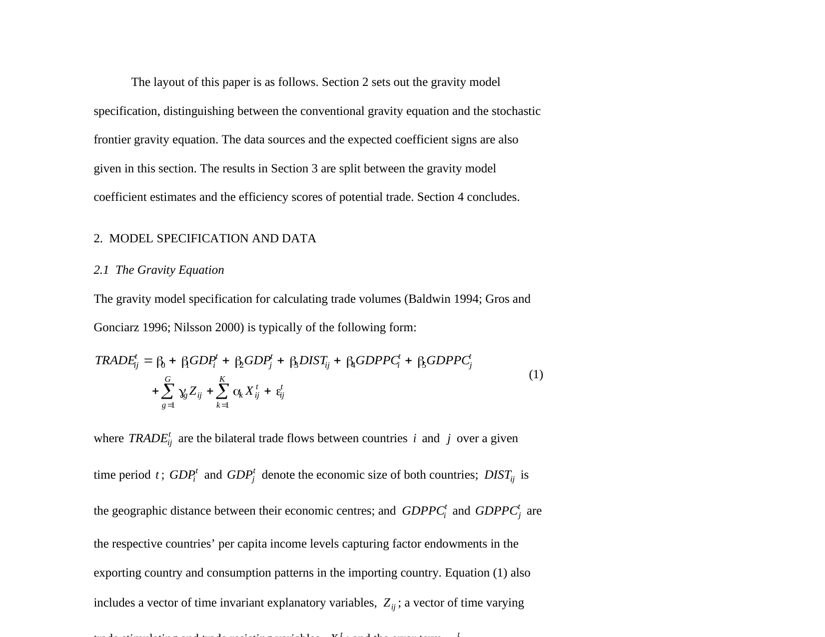
The layout of this paper is as follows. Section 2 sets out the gravity model
specification, distinguishing between the conventional gravity equation and the stochastic
frontier gravity equation. The data sources and the expected coefficient signs are also
given in this section. The results in Section 3 are split between the gravity model
coefficient estimates and the efficiency scores of potential trade. Section 4 concludes.
2. MODEL SPECIFICATION AND DATA
2.1 The Gravity Equation
The gravity model specification for calculating trade volumes (Baldwin 1994; Gros and
Gonciarz 1996; Nilsson 2000) is typically of the following form:
t
j
t
iij
t
j
t
i
t
ij GDPPCGDPPCDISTGDPGDPTRADE 543210  
t
ij
K
k
t
ijk
G
g
ijg XZ     11
(1)
where t
ijTRADE are the bilateral trade flows between countries i and j over a given
time period t ; t
iGDP and t
jGDP denote the economic size of both countries; ijDIST is
the geographic distance between their economic centres; and t
iGDPPC and t
jGDPPC are
the respective countries’ per capita income levels capturing factor endowments in the
exporting country and consumption patterns in the importing country. Equation (1) also
includes a vector of time invariant explanatory variables, ijZ ; a vector of time varying

trade is defined relative to the sample average rather than in terms of a maximum level
feasible for a given pair of trading partners. Measuring trade potential against mean
predicted values can be problematic because the predictive ability of the gravity model
declines as the year of the inserted values increasingly deviates from the sample average. 2
Under the stochastic frontier analysis (SFA) approach, the gravity equation of
trade determinants identifies the trade frontier. The resulting frontier levels of trade, i.e.
the maximum possible level of trade for a given bilateral trading pair, is impacted by a
random error term which can be positive or negative thereby allowing the stochastic
frontier trade level to vary about the deterministic part of the gravity equation. Observed
trade levels can then be compared against this frontier level of trade for each bilateral
trading pair to assess the scope for trade expansion. The next section provides a detailed
exposition of this approach.
2.2 The Gravity Equation estimated using Stochastic Frontier Analysis
Developed independently by Aigner et al. (1977) and Meeusen and van den Broeck
(1977), stochastic frontier analysis (SFA) has been used extensively in the assessment of
firm performance. In its traditional application, SFA specifies a production frontier
representing the maximum output that can be produced from a given level of inputs.
Fully efficient firms operate on the frontier such that observed and frontier levels of
output coincide, while (technically) inefficient firms operate at a point within the frontier,
signifying a shortfall between the observed and the maximum possible levels of output.

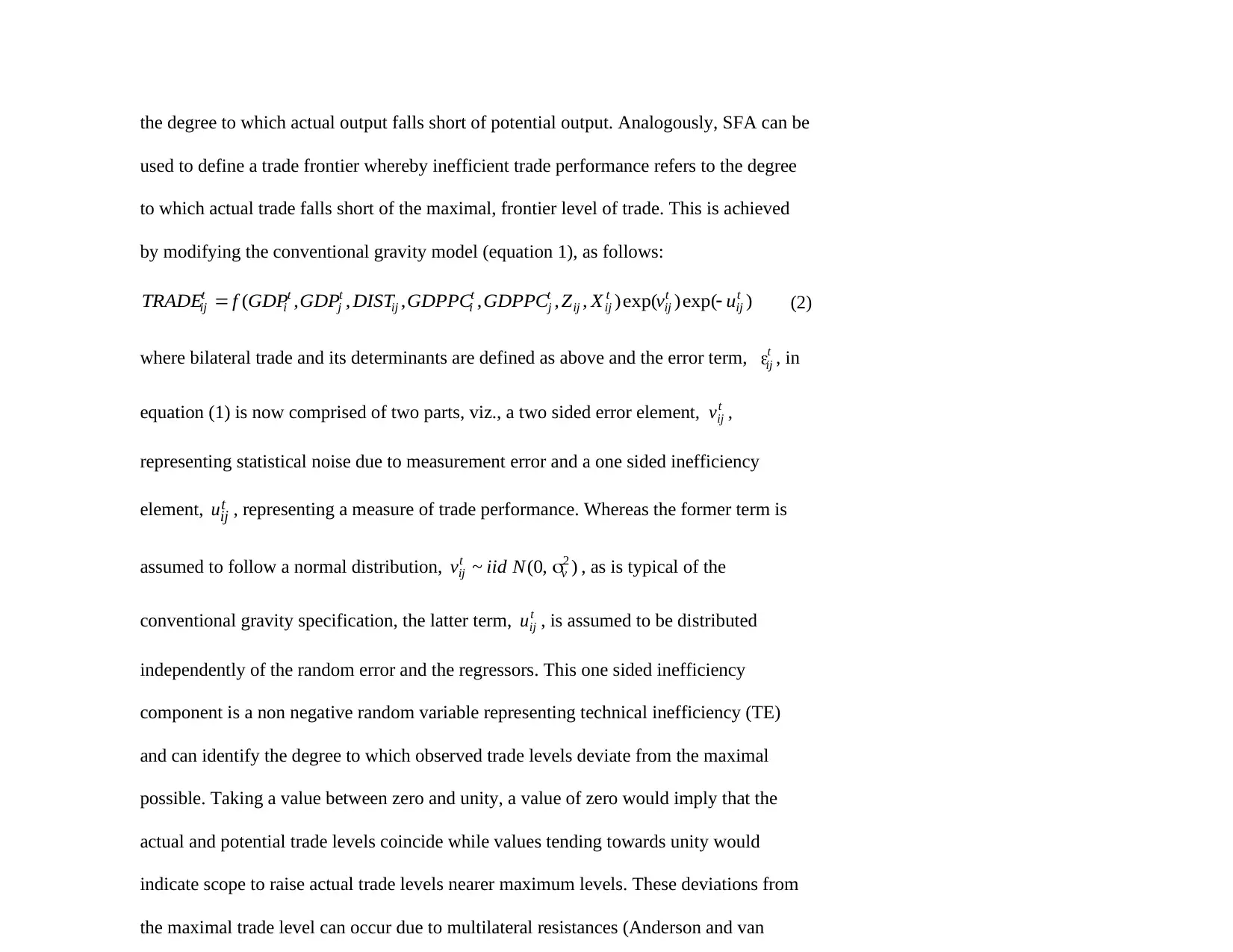
the degree to which actual output falls short of potential output. Analogously, SFA can be
used to define a trade frontier whereby inefficient trade performance refers to the degree
to which actual trade falls short of the maximal, frontier level of trade. This is achieved
by modifying the conventional gravity model (equation 1), as follows:
)exp()exp(),,,,,,( t
ij
t
ij
t
ijij
t
j
t
iij
t
j
t
i
t
ij uvXZGDPPCGDPPCDISTGDPGDPfTRADE  (2)
where bilateral trade and its determinants are defined as above and the error term, t
ij , in
equation (1) is now comprised of two parts, viz., a two sided error element, t
ijv ,
representing statistical noise due to measurement error and a one sided inefficiency
element, t
iju , representing a measure of trade performance. Whereas the former term is
assumed to follow a normal distribution, ),0(~ 2
v
t
ij Niidv  , as is typical of the
conventional gravity specification, the latter term, t
iju , is assumed to be distributed
independently of the random error and the regressors. This one sided inefficiency
component is a non negative random variable representing technical inefficiency (TE)
and can identify the degree to which observed trade levels deviate from the maximal
possible. Taking a value between zero and unity, a value of zero would imply that the
actual and potential trade levels coincide while values tending towards unity would
indicate scope to raise actual trade levels nearer maximum levels. These deviations from
the maximal trade level can occur due to multilateral resistances (Anderson and van

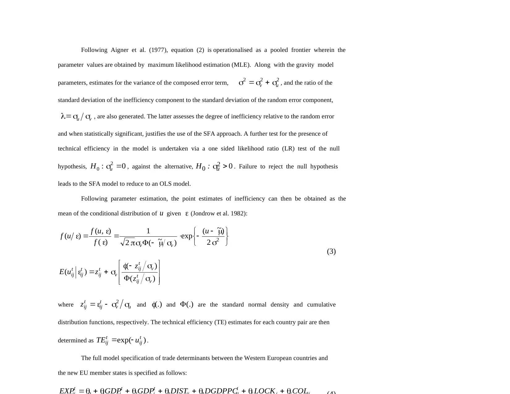
Following Aigner et al. (1977), equation (2) is operationalised as a pooled frontier wherein the
parameter values are obtained by maximum likelihood estimation (MLE). Along with the gravity model
parameters, estimates for the variance of the composed error term, 222
uv   , and the ratio of the
standard deviation of the inefficiency component to the standard deviation of the random error component,
vu  , are also generated. The latter assesses the degree of inefficiency relative to the random error
and when statistically significant, justifies the use of the SFA approach. A further test for the presence of
technical efficiency in the model is undertaken via a one sided likelihood ratio (LR) test of the null
hypothesis, 0: 2
0 uH  , against the alternative, 02
0 u:H  . Failure to reject the null hypothesis
leads to the SFA model to reduce to an OLS model.
Following parameter estimation, the point estimates of inefficiency can then be obtained as the
mean of the conditional distribution of u given  (Jondrow et al. 1982):





 


 2
2
)~(
exp
)~(2
1
)(
),(
)( 



 u
f
uf
uf
vv
)(
)(
)(











v
t
ij
v
t
ij
v
t
ij
t
ij
t
ij z
z
zuE 


(3)
where uv
t
ij
t
ijz  2
 and (.) and (.) are the standard normal density and cumulative
distribution functions, respectively. The technical efficiency (TE) estimates for each country pair are then
determined as )exp( t
ij
t
ij uTE  .
The full model specification of trade determinants between the Western European countries and
the new EU member states is specified as follows:
tttt COLLOCKDGDPPCDISTGDPGDPEXP  

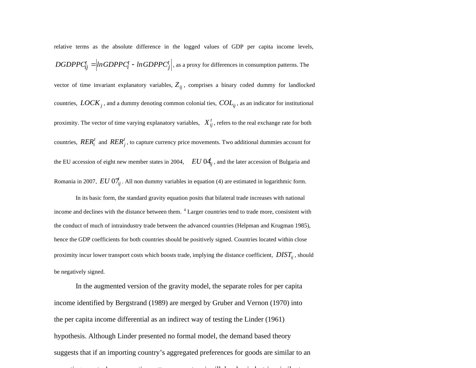
relative terms as the absolute difference in the logged values of GDP per capita income levels,
tj
t
i
t
ij GDPPClnGDPPClnDGDPPC  , as a proxy for differences in consumption patterns. The
vector of time invariant explanatory variables, ijZ , comprises a binary coded dummy for landlocked
countries, jLOCK , and a dummy denoting common colonial ties, ijCOL , as an indicator for institutional
proximity. The vector of time varying explanatory variables, t
ijX , refers to the real exchange rate for both
countries, t
iRER and t
jRER , to capture currency price movements. Two additional dummies account for
the EU accession of eight new member states in 2004, t
ijEU 04 , and the later accession of Bulgaria and
Romania in 2007, t
ijEU 07 . All non dummy variables in equation (4) are estimated in logarithmic form.
In its basic form, the standard gravity equation posits that bilateral trade increases with national
income and declines with the distance between them. 4 Larger countries tend to trade more, consistent with
the conduct of much of intraindustry trade between the advanced countries (Helpman and Krugman 1985),
hence the GDP coefficients for both countries should be positively signed. Countries located within close
proximity incur lower transport costs which boosts trade, implying the distance coefficient, ijDIST , should
be negatively signed.
In the augmented version of the gravity model, the separate roles for per capita
income identified by Bergstrand (1989) are merged by Gruber and Vernon (1970) into
the per capita income differential as an indirect way of testing the Linder (1961)
hypothesis. Although Linder presented no formal model, the demand based theory
suggests that if an importing country’s aggregated preferences for goods are similar to an

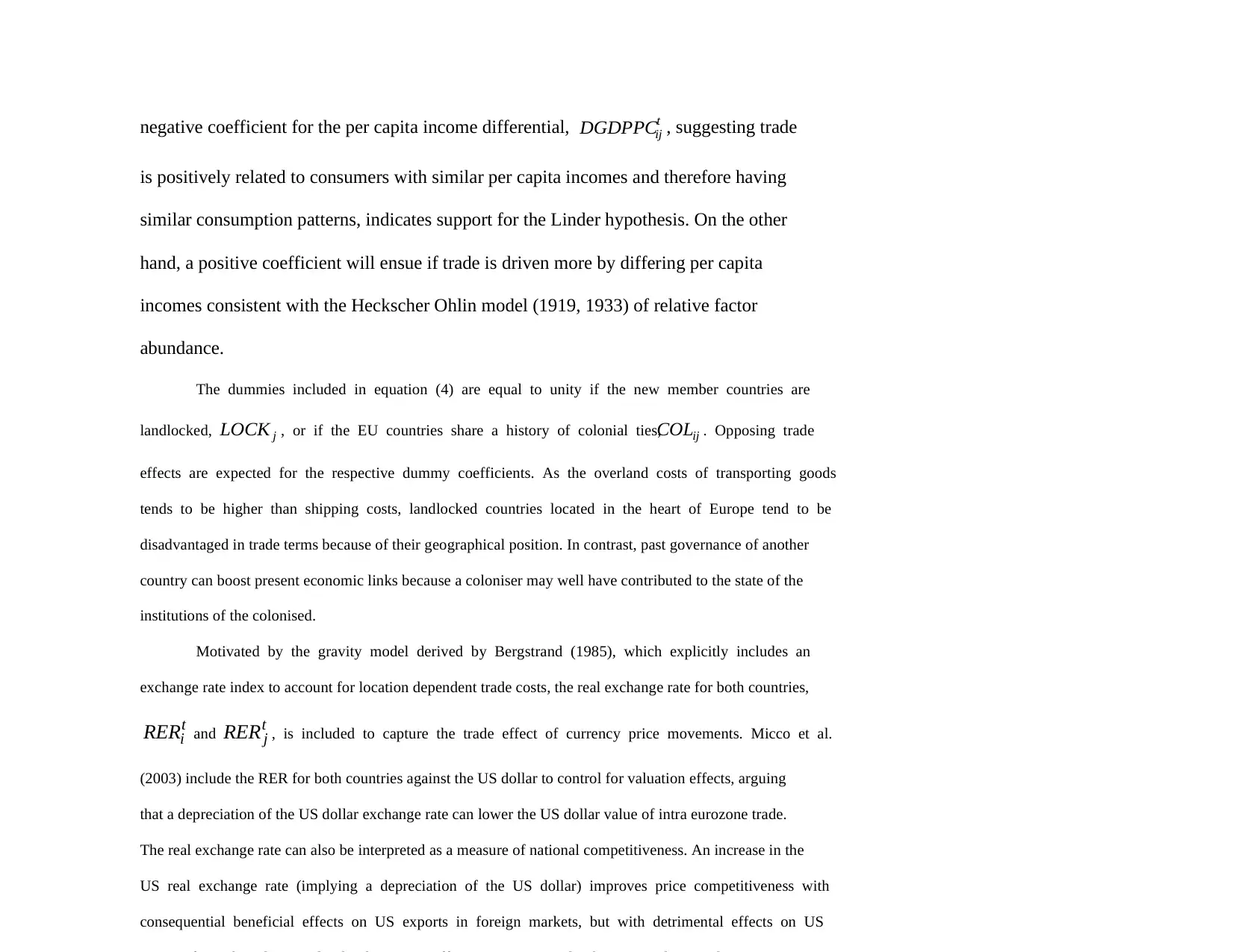
negative coefficient for the per capita income differential, t
ijDGDPPC , suggesting trade
is positively related to consumers with similar per capita incomes and therefore having
similar consumption patterns, indicates support for the Linder hypothesis. On the other
hand, a positive coefficient will ensue if trade is driven more by differing per capita
incomes consistent with the Heckscher Ohlin model (1919, 1933) of relative factor
abundance.
The dummies included in equation (4) are equal to unity if the new member countries are
landlocked, jLOCK , or if the EU countries share a history of colonial ties, ijCOL . Opposing trade
effects are expected for the respective dummy coefficients. As the overland costs of transporting goods
tends to be higher than shipping costs, landlocked countries located in the heart of Europe tend to be
disadvantaged in trade terms because of their geographical position. In contrast, past governance of another
country can boost present economic links because a coloniser may well have contributed to the state of the
institutions of the colonised.
Motivated by the gravity model derived by Bergstrand (1985), which explicitly includes an
exchange rate index to account for location dependent trade costs, the real exchange rate for both countries,
t
iRER and tjRER , is included to capture the trade effect of currency price movements. Micco et al.
(2003) include the RER for both countries against the US dollar to control for valuation effects, arguing
that a depreciation of the US dollar exchange rate can lower the US dollar value of intra eurozone trade.
The real exchange rate can also be interpreted as a measure of national competitiveness. An increase in the
US real exchange rate (implying a depreciation of the US dollar) improves price competitiveness with
consequential beneficial effects on US exports in foreign markets, but with detrimental effects on US