GWAS Summary Statistics Imputation using FIZI on UKBiobank Data

This project investigates the imputation of unmeasured genome-wide association study (GWAS) summary statistics using various statistical methods on the UKBiobank dataset. It employs Functionally-informed Z-score Imputation (FIZI) to impute GWAS summary statistics, leveraging linkage disequilibrium (LD) data. The study compares FIZI's performance with the traditional ImpG method and explores alternative approaches using LDSC and PolyFun to extract effect sizes. By analyzing 22 chromosomes, the project evaluates the accuracy and precision of imputing unmeasured markers, comparing penalized and unpenalized LD regressions. The goal is to enhance the imputation process and improve the understanding of genetic variations in complex traits.

Project 3
Abstract
Recent work has performed various statistical methods to impute unmeasured genome-
wide association study (GWAS) summary statistics and demonstrated a path to
overcome the challenges of imputing individual-level genetic variation with a precise
result. In this project, we used various approaches to make imputation in a genome
regards the unmeasured markers utilizing the information from the measure markers.
We analyzed the 22 chromosomes of each individual in the UKBiobank dataset and
discovered the taus coefficients. Functionally-informed Z-score Imputation (FIZI) was
introduced to impute GWAS summary statistics (Z-score) on the unmeasured markers
by leveraging data with linkage-disequilibrium (LD) when prior taus are known. The old
method for such imputation that is used for many years is called ImpG, whereas it takes
no prior variance in the imputation. Recent studies have proposed an alternative
approach, that is extracting the effect sizes taus coefficients directly from the SNP Chip
and imputing the new observed effect sizes with Reference Panel Whole Genome
Sequencing. To test for accuracy and precision, here we use the observed information
of the measured markers plus the reference panel from two methods: LDSC and
PolyFun. We retrieve the taus scores with penalized LD regressions by running
Polygenic Functionally-informed fine-mapping (PolyFun), and taus scores with
unpenalized LD regressions by running LD Score Regression (LDSC). We compare
with the distribution of residuals along with the Z summary statistics with the traditional
model ImpG, to determine the performance in whether estimating the summary
statistics with penalized or unpenalized LD regressions are performing better than the
conventional method ImpG.
1. Introduction
Overview:
Genome-wide association study, also known as the whole genome-wide association
study, is an approach in which scientists used to identify the specific genetic
associations in genetic research. In GWAS, things that we usually look at are major
allele, minor allele, etc. and the metrics that we apply more with are linkage
disequilibrium (LD). The study of genetics is the prime study that will help in the
determination of the variants of genomes. The genome-wide association study focuses
on the behavior of the human DNA that will help in the decision of the genes and
identification of diseases. The GWAS studies the DNA that performs differently, or the
DNA of participants has a different phenotype for the understanding of a particular
disease or a trait. GWAS discovers the development of the DNA, which helps in the
knowledge of illnesses and behavior of humans. In other words, it can be said that the
Genome-wide association study is the study that helps in the identification of the
changes that have been brought in the traits or characteristics of human DNA due to
changes in the environment.

In GWAS of complex traits, a high percentage of heritability can be analyzed and
explained within single nucleotide polymorphisms (SNP). Many of the GWAS studies
are conducted through Meta-analysis but not necessarily carry out the summary
statistics for individual genome. When there are unmeasured alleles in an association
study, we use the information on the LD pattern relating to the measured markers to
impute the unmeasured markers. GWAS relies on genotype imputation where the
unmeasured markers are predicted and estimated by referencing a large scale of
panels of sequenced individuals. The primary computation source that was used to
calculate unmeasured GWAS summary statistics is linkage-disequilibrium, which could
be obtained from different publicly available reference genome panels. Summary-based
statistics are often used to summarize considerate information such as central tendency
and measure of spread and proved to be highly accurate, stable, and within each
genotype data.
The dataset we used to demonstrate our idea is called UKBiobank. The dataset
recruited 500,000 people ages 40 to 69 years in 2006-2010 from across the country. In
our work, we attempt to establish a statistical model to impute GWAS summary
statistics by leveraging functional data. We make an imputation on the linkage-
disequilibrium among the unmeasured markers to obtain sufficient summary statistics.
Our approach is to apply Functionally-informed Z-score Imputation (FIZI) to form a
linear model based on LD-weighted statistics with annotations. To test for accuracy and
precision, before running FIZI, we have a different approach: retrieving the taus score
with an L2-regularized S-LD score by running Polygenic Functionally-informed fine-
mapping (PolyFun). PolyFun estimates prior causal probability for SNPs that can be
used by fine-mapping methods. PolyFun can also aggregate polygenic data from across
the entire genome and hundreds of functional annotations. Our goal is to examine the
association upon the variance of the measured markers within each SNP between the
two approaches and observe whether the penalized LD scores are shown to make a
significant difference. With the results from LD score estimation, we aim to improve the
power when performing FIZI on the prior taus estimation from Polyfun.
2 Methods
 Overview of the methods
For real data analysis, we applied FIZI, ImpG, and PolyFun to GWAS summary
statistics gathered from approximately 337k individuals of European ancestry in the UK
Biobank with 22 complex traits. Our analysis based on the assumption that the models
summary statistics are under a linear model. The FIZI model performed the imputation
on the given GWAS summary statistics Zo (measured markers) with linkage
disequilibrium and variance estimates. Assuming the model is linear, and SNP effect
sizes are drawn from a normal distribution with variance defined by functional
categories, we model the unobserved summary data Zu under a conditional normal
form as:
Zu | Zo ~ N(Vu,oVo,oZo, Vu,u – Vu,oVo,oVo,u)

Where Vu,o = Σu,o + Σu,uDu,uΣu,o + Σu,o+Do,oΣo,o
Vo,o = Σo,o + Σo,oDo,oΣo,o + Σo,u+Du,uΣu,o
And Σ denotes the linkage disequilibrium and D dontes the variance estimates.
When running ImpG using FIZI, the LD score in the model is unpenalized, which could
potentially bring noises and conservative in power in estimating the taus. To test for the
differences, here, we will use an additional procedure to evaluate the GWAS summary
statistics of the variations within the SNPs. PolyFun is appointed to impute taus using
the penalized LD score regression. The data frame is still the same as FIZI linear
model, and with this approach, we are hoping to get the summary statistics on the
penalized taus that is more precise and closer to 0.
 Polyfun output
Under the same condition normal frame, we retrieve the taus score by running PolyFun
on the data. The goal of running PolyFun is to estimate the prior causal probability for
SNPs across the entire genome and hundreds of functional annotations. We create the
residuals plot to assess the association between the two methods on the taus. The
result is convincing that the two approaches illustrate differences statistically. Here are
some plots extracted from 27 traits:
We graph the scenario and displayed it in a scatter plot along with a reference line to
indicate the trending. These plots suggest that as the majority of the points do fall
around the reference line, but there are also a couple of outliers relatively far away from
the reference. Using the summary statistics retrieving from PolyFun, we proceed to
impute FIZI on the taus.
 Measure of accuracy
Given the linear matrix model in the output of the PolyFun frame, we compute the
measure of accuracy based on the measure of R2. The imputation accuracy R2 is
bounded from 0 to 1, and to account for variance due to random effects, or noises, we
propose:
Where we dropped the conditioned parameters to simplify notation. The R square here
captures the notation of R2 measure that is 1 minus the ratio of residual variance versus
total variance.

3 Results
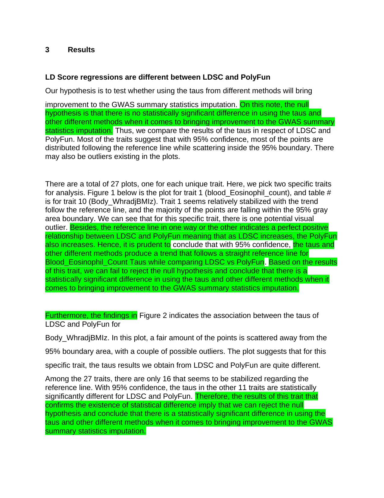
LD Score regressions are different between LDSC and PolyFun
Our hypothesis is to test whether using the taus from different methods will bring
improvement to the GWAS summary statistics imputation. On this note, the null
hypothesis is that there is no statistically significant difference in using the taus and
other different methods when it comes to bringing improvement to the GWAS summary
statistics imputation. Thus, we compare the results of the taus in respect of LDSC and
PolyFun. Most of the traits suggest that with 95% confidence, most of the points are
distributed following the reference line while scattering inside the 95% boundary. There
may also be outliers existing in the plots.
There are a total of 27 plots, one for each unique trait. Here, we pick two specific traits
for analysis. Figure 1 below is the plot for trait 1 (blood_Eosinophil_count), and table #
is for trait 10 (Body_WhradjBMIz). Trait 1 seems relatively stabilized with the trend
follow the reference line, and the majority of the points are falling within the 95% gray
area boundary. We can see that for this specific trait, there is one potential visual
outlier. Besides, the reference line in one way or the other indicates a perfect positive
relationship between LDSC and PolyFun meaning that as LDSC increases, the PolyFun
also increases. Hence, it is prudent to conclude that with 95% confidence, the taus and
other different methods produce a trend that follows a straight reference line for
Blood_Eosinophil_Count Taus while comparing LDSC vs PolyFun. Based on the results
of this trait, we can fail to reject the null hypothesis and conclude that there is a
statistically significant difference in using the taus and other different methods when it
comes to bringing improvement to the GWAS summary statistics imputation.
Furthermore, the findings in Figure 2 indicates the association between the taus of
LDSC and PolyFun for
Body_WhradjBMIz. In this plot, a fair amount of the points is scattered away from the
95% boundary area, with a couple of possible outliers. The plot suggests that for this
specific trait, the taus results we obtain from LDSC and PolyFun are quite different.
Among the 27 traits, there are only 16 that seems to be stabilized regarding the
reference line. With 95% confidence, the taus in the other 11 traits are statistically
significantly different for LDSC and PolyFun. Therefore, the results of this trait that
confirms the existence of statistical difference imply that we can reject the null
hypothesis and conclude that there is a statistically significant difference in using the
taus and other different methods when it comes to bringing improvement to the GWAS
summary statistics imputation.

Figure 1 Blood_Eosinophil_Count Taus Comparison LDSC vs PolyFun

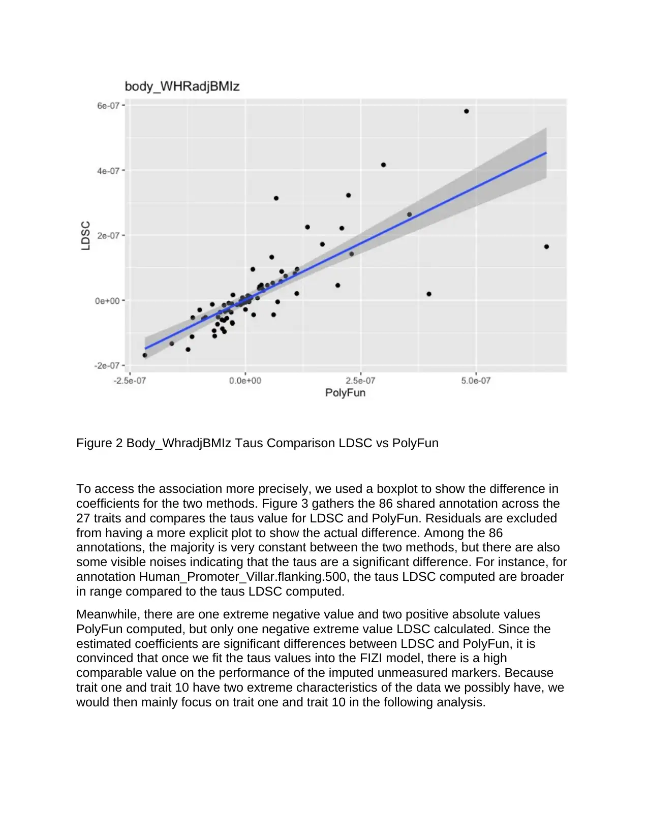
Figure 2 Body_WhradjBMIz Taus Comparison LDSC vs PolyFun
To access the association more precisely, we used a boxplot to show the difference in
coefficients for the two methods. Figure 3 gathers the 86 shared annotation across the
27 traits and compares the taus value for LDSC and PolyFun. Residuals are excluded
from having a more explicit plot to show the actual difference. Among the 86
annotations, the majority is very constant between the two methods, but there are also
some visible noises indicating that the taus are a significant difference. For instance, for
annotation Human_Promoter_Villar.flanking.500, the taus LDSC computed are broader
in range compared to the taus LDSC computed.
Meanwhile, there are one extreme negative value and two positive absolute values
PolyFun computed, but only one negative extreme value LDSC calculated. Since the
estimated coefficients are significant differences between LDSC and PolyFun, it is
convinced that once we fit the taus values into the FIZI model, there is a high
comparable value on the performance of the imputed unmeasured markers. Because
trait one and trait 10 have two extreme characteristics of the data we possibly have, we
would then mainly focus on trait one and trait 10 in the following analysis.

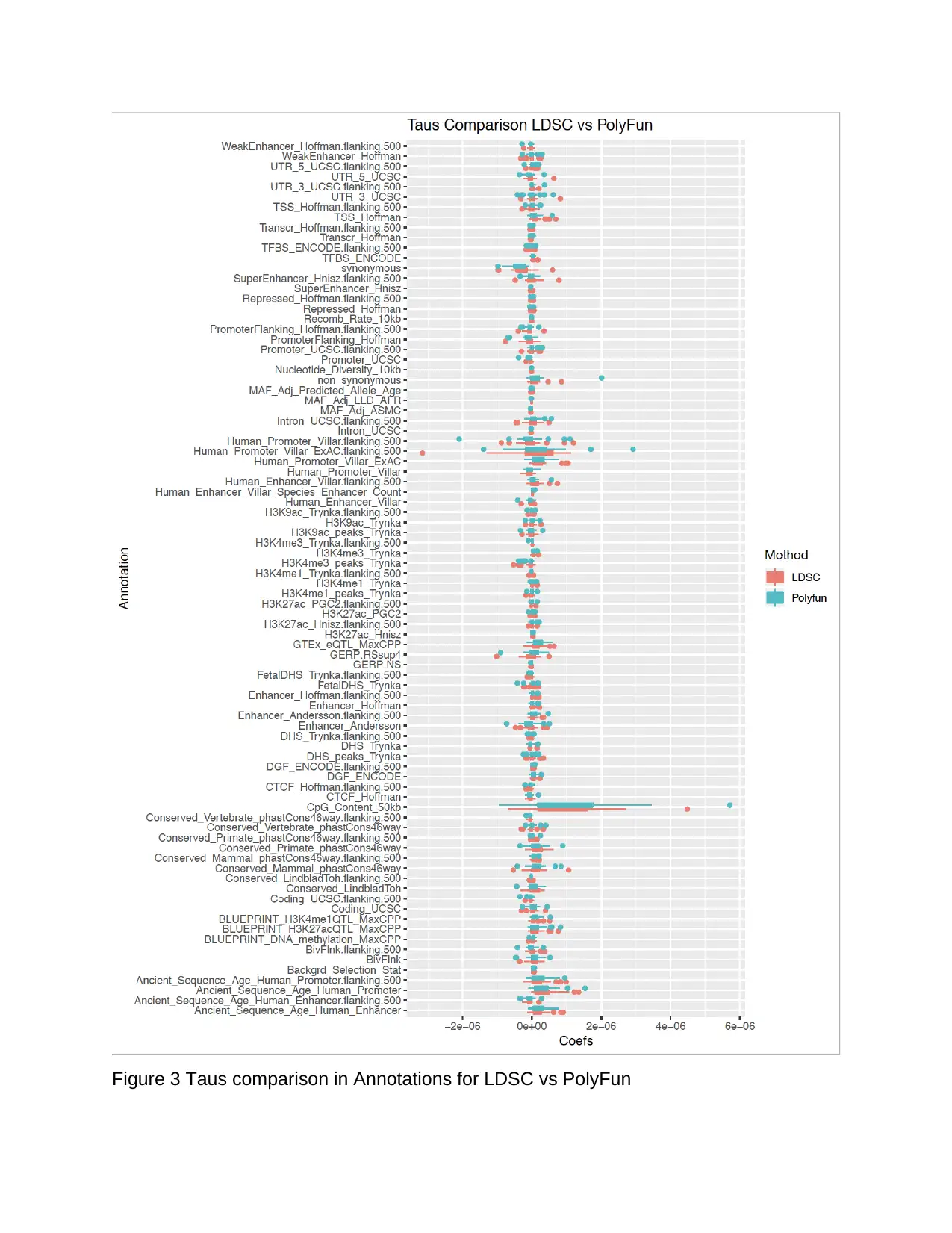
Figure 3 Taus comparison in Annotations for LDSC vs PolyFun

FIZI accurately imputes GWAS summary statistics
To ascertain the statistically significant difference in using the taus and other different
methods when it comes to bringing improvement to the GWAS summary statistics
imputation, we assess the performance of FIZI using simulated GWAS summary
statistics when prior taus values are known by sampling Z-scores Z statistics under
multiple genome parameters at each region. The summary statistics result is proved to
be accurate after comparing it with the unaware approach, ImpG. Similarly, the Z-scores
Z statistics under multiple genome parameters at each region are expected not to give
similar results and this will show the actual difference between the taus and other
different methods while improving the GWAS summary statistics imputation. Hence,
giving a statistical decision based on the outputs.
When prior τs are known, FIZI outperformed ImpG across all tested proportions
exhibiting a mean R2 between the true and predicted Z-scores of 0.97 for FIZI compared
with 0.96 for ImpG. In other words, FIZI gives an accurate prediction of the model to be
97% compared to ImpG whose accurate level of model prediction is 96%. However, the
results on the τs are not so good as the τs are noisy. Here, we apply with PolyFun to
obtain the penalized τs in the LD regression, aiming to improve the power of the
summary statistics on the τs.
Imputed GWAS summary statistics by using FIZI with ImpG, LDSC, and PolyFun
As mentioned in the method section, FIZI automatically imputes the ImpG result when
no taus value is fitted into the model. We retrieve the imputed summary statistics for
LDSC and PolyFun by providing the taus values into the FIZI model. For each Z
statistics we obtained in 3 different approaches, we compare with the original summary
statistics downloaded at
and get the R square. R square bounded from 0 to 1, with higher the value indicating
the more robust the association. If an R square value is equal to 1, that means our likely
result with that specific method has correctly predicted the result compare with the
original summary statistics.
The results are quite surprising as PolyFun with the penalized taus are far off on the left
across 22 chromosomes, indicating that the imputed summary statistics have a fragile
association with the original summary statistics. When estimating the R square, we are
hoping to see values that are relatively close to positive 1. Recall that when we were
contrasting the imputed taus between LDSC and PolyFun, trait1
Blood_Eosinophil_Count Taus is very stabilized, and the distribution follows the
regression reference line. The fact is, across the 22 chromosomes, PolyFun is
essentially performing better than LDSC, specifically for trait 1.
LDSC seems to be more accurate in general than PolyFun in predicting the Z score as
most of the R square values are above 0.6. Recall that in the taus comparison plot trait
10, Body_WhradjBMIz has a wild distribution, and most of the points are scattered

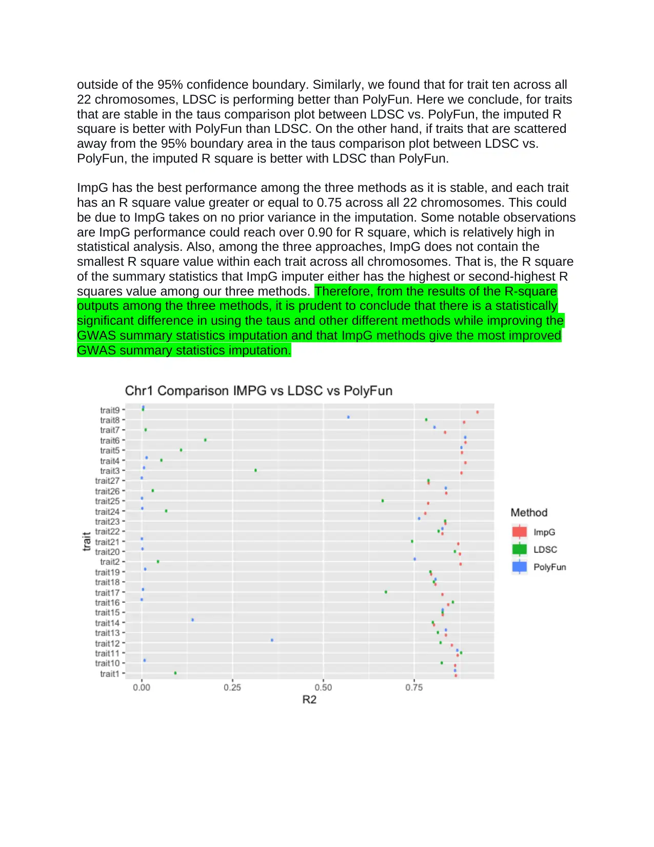
outside of the 95% confidence boundary. Similarly, we found that for trait ten across all
22 chromosomes, LDSC is performing better than PolyFun. Here we conclude, for traits
that are stable in the taus comparison plot between LDSC vs. PolyFun, the imputed R
square is better with PolyFun than LDSC. On the other hand, if traits that are scattered
away from the 95% boundary area in the taus comparison plot between LDSC vs.
PolyFun, the imputed R square is better with LDSC than PolyFun.
ImpG has the best performance among the three methods as it is stable, and each trait
has an R square value greater or equal to 0.75 across all 22 chromosomes. This could
be due to ImpG takes on no prior variance in the imputation. Some notable observations
are ImpG performance could reach over 0.90 for R square, which is relatively high in
statistical analysis. Also, among the three approaches, ImpG does not contain the
smallest R square value within each trait across all chromosomes. That is, the R square
of the summary statistics that ImpG imputer either has the highest or second-highest R
squares value among our three methods. Therefore, from the results of the R-square
outputs among the three methods, it is prudent to conclude that there is a statistically
significant difference in using the taus and other different methods while improving the
GWAS summary statistics imputation and that ImpG methods give the most improved
GWAS summary statistics imputation.

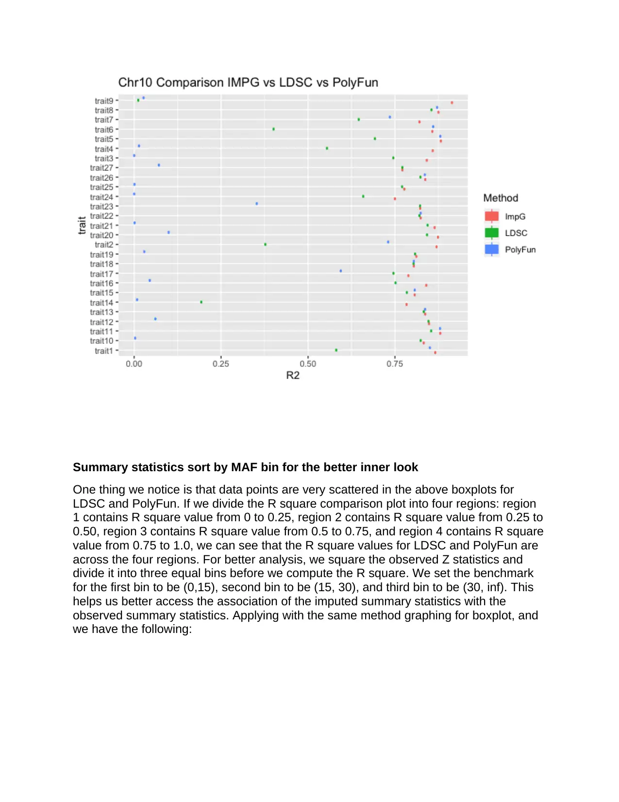
Summary statistics sort by MAF bin for the better inner look
One thing we notice is that data points are very scattered in the above boxplots for
LDSC and PolyFun. If we divide the R square comparison plot into four regions: region
1 contains R square value from 0 to 0.25, region 2 contains R square value from 0.25 to
0.50, region 3 contains R square value from 0.5 to 0.75, and region 4 contains R square
value from 0.75 to 1.0, we can see that the R square values for LDSC and PolyFun are
across the four regions. For better analysis, we square the observed Z statistics and
divide it into three equal bins before we compute the R square. We set the benchmark
for the first bin to be (0,15), second bin to be (15, 30), and third bin to be (30, inf). This
helps us better access the association of the imputed summary statistics with the
observed summary statistics. Applying with the same method graphing for boxplot, and
we have the following:

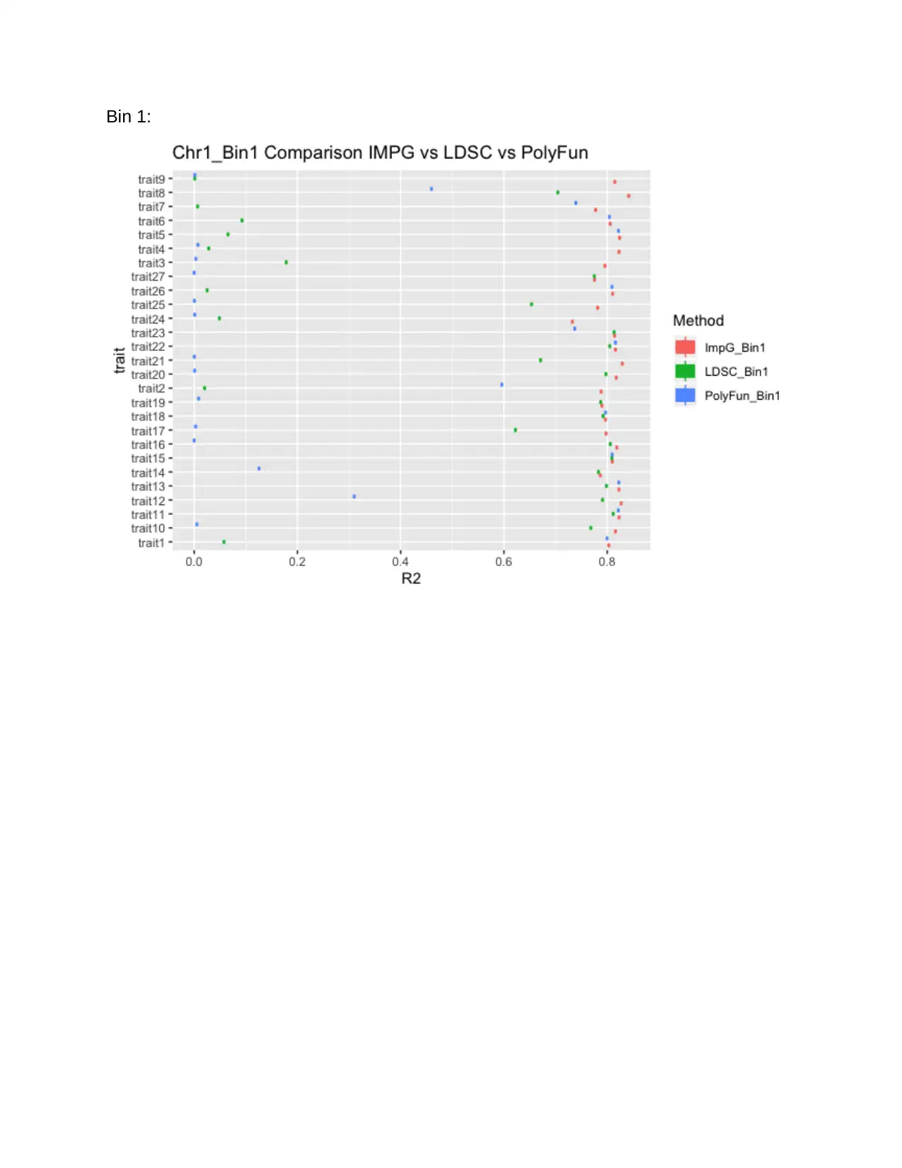
Bin 1:

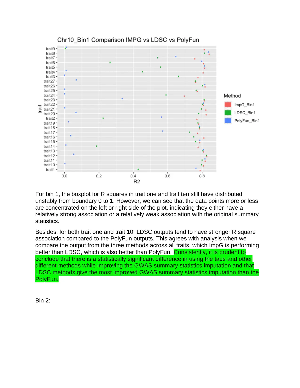
For bin 1, the boxplot for R squares in trait one and trait ten still have distributed
unstably from boundary 0 to 1. However, we can see that the data points more or less
are concentrated on the left or right side of the plot, indicating they either have a
relatively strong association or a relatively weak association with the original summary
statistics.
Besides, for both trait one and trait 10, LDSC outputs tend to have stronger R square
association compared to the PolyFun outputs. This agrees with analysis when we
compare the output from the three methods across all traits, which ImpG is performing
better than LDSC, which is also better than PolyFun. Consistently, it is prudent to
conclude that there is a statistically significant difference in using the taus and other
different methods while improving the GWAS summary statistics imputation and that
LDSC methods give the most improved GWAS summary statistics imputation than the
PolyFun.
Bin 2: