Statistics Summary Report: Analysis of Healthcare Access in SBS 2000

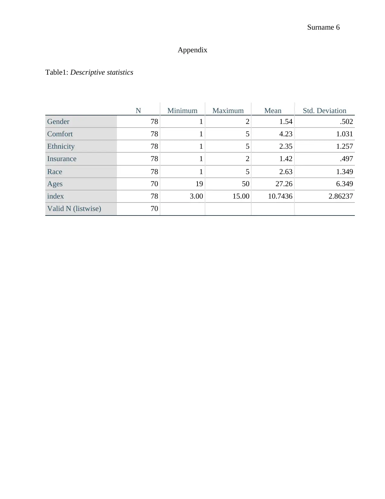
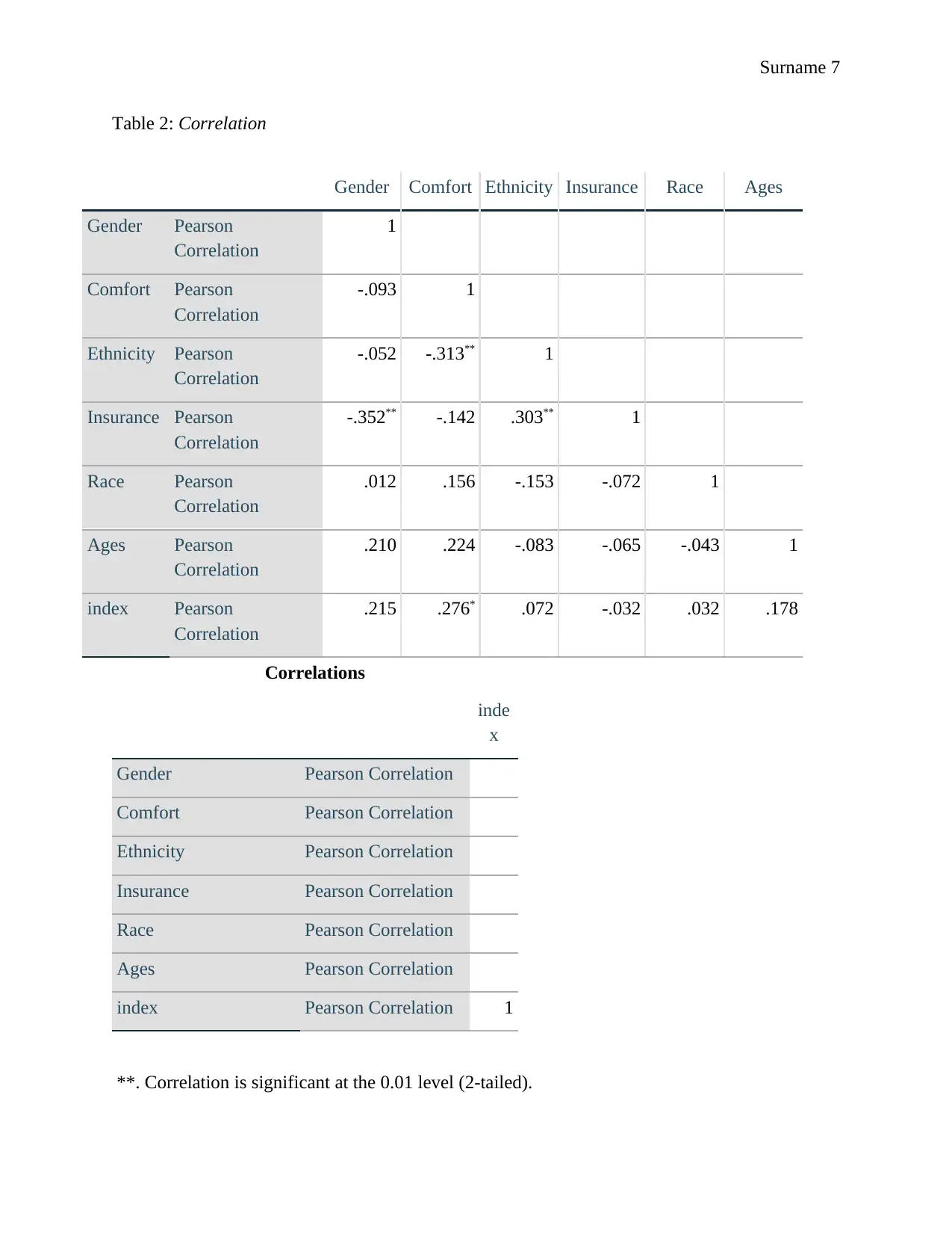
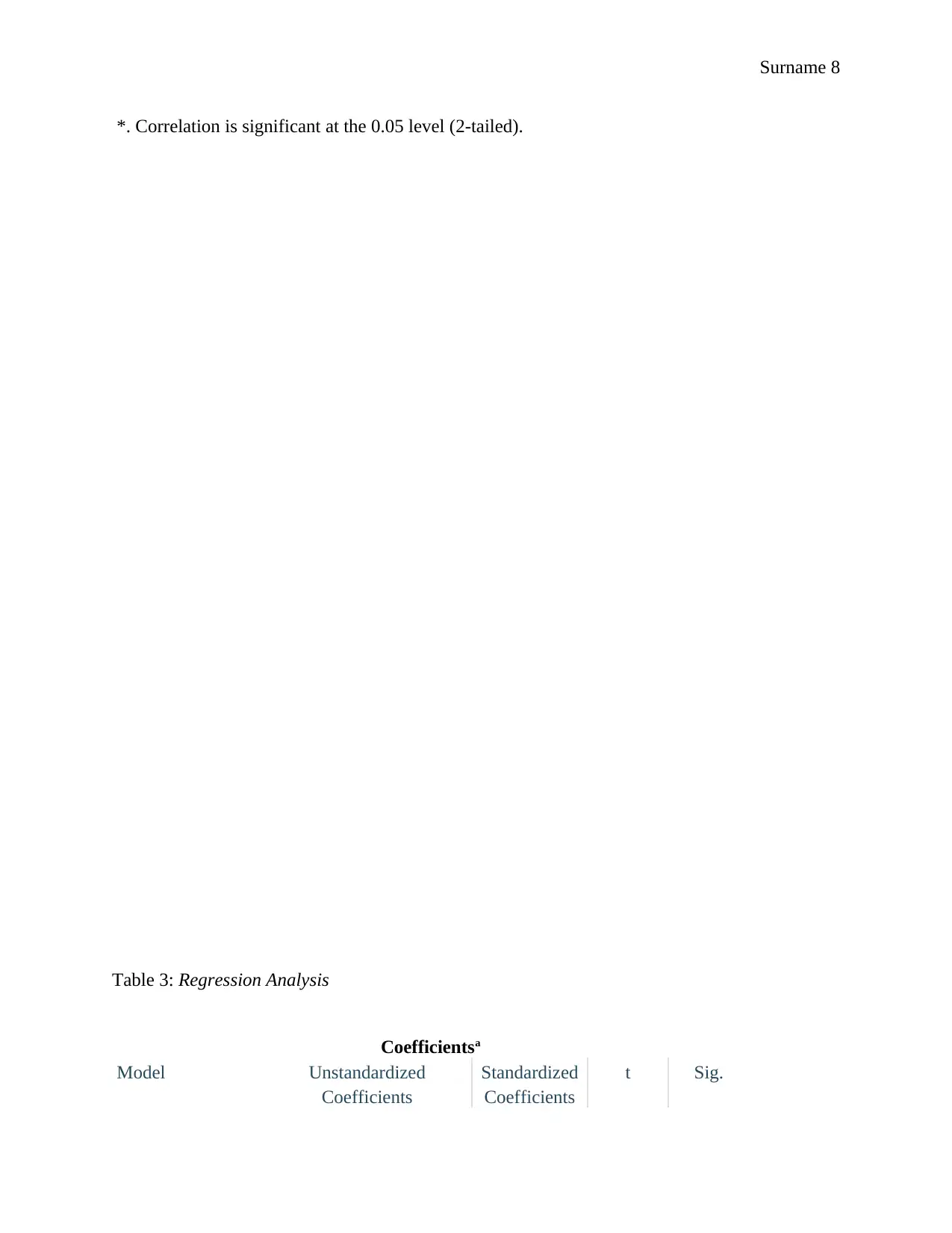
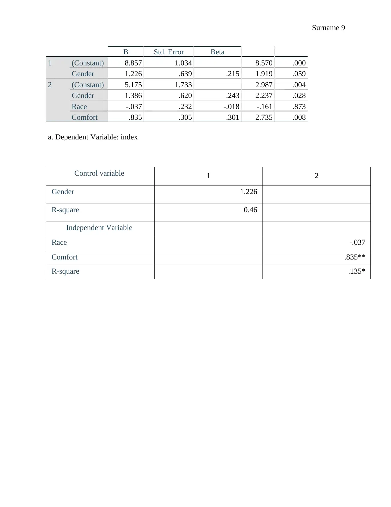
This report presents a statistical analysis of healthcare access, incorporating descriptive statistics, correlation analysis, and regression modeling. The study utilizes data on gender, comfort, ethnicity, insurance, race, age, and an index of access, employing Pearson's correlation coefficient to assess relationships between variables. Linear regression models were developed to explore the impact of gender, race, and comfort on the index. Findings reveal that approximately 46% of the variation in the index is attributable to these variables. The report tests hypotheses regarding the impact of gender, race, and comfort on the index, concluding that gender and comfort have significant effects, while race does not. The analysis includes detailed tables of descriptive statistics, correlation matrices, and regression coefficients. The student used the information in the assignment brief, which included the dependent and independent variables and the questions used to measure them. The student also provided the coding for the variables.

Surname 1
Student’s Name
Instructor’s Name
Course Number
Date Submitted
Statistics Summary Report
Descriptive Statistics
To establish the characteristics of the variables in the dataset, summary statistics were
obtained, and the results were as shown in Table 1 (Appendix). Table 1 can be used to examine
the variability of each variable in the study by comparing its mean to the corresponding standard
deviation. From statistical theory, if the mean of a variable is higher than its standard deviation,
then there exists a lower variability of variables within the mean. On the contrary, a standard
deviation that exceeds the mean implies that there is a higher variation. From the table, it is
evident that the mean value of each variable exceeded the standard deviation; hence there was
low variability in the recorded values. In particular, the means (and standard deviations) of each
of the variables were: gender 1.54 (0.52), comfort 4.23 (1.031), ethnicity 2.35 (1.257), insurance
1.42 (0.497), race 2.63 (1.349), ages 27.26 (6.349), and index 10.7436 (2.86237).
Correlation Analysis
In this study, the variable gender was transformed into a numeric value. Pearson’s
coefficient can be adopted in analyses that involve numeric data (Akoglu, 92). Since the
remaining variables were numeric, Pearson’s correlation coefficient was adopted, and the
outcomes were summarized in Table 2 (Appendix). From the table, none of the possible pairs of

Surname 2
variables have a correlation coefficient that is greater than 0.8; hence, it can be deduced that
there is no multicollinearity. Also, Table 2 indicates that there exist weak associations between
pairs of variables since none of the coefficients is equal to or greater than 0.5.
Regression Analysis
Linear regression a reliable model for exploring the association between two or more
variables (Aggarwal & Ranganathan, 101). Ordinarily, one variable is regarded as a result,
whose occurrence is contingent on two or more other variables. Consequently, regression
analysis is a statistical approach for exploring the extent to which the dependent variable is
affected by some identified independent predictors (Aggarwal & Ranganathan, 101).
Denoting the outcome as y, the corresponding predictors can be denoted by x1, x2, …, xn.
The linear model that can be used to explain the association between the former and the latter
categories of variables is of the form:
y = β + β₀ 1x1 + β2x2 + … + βnxn (Li et al., 926).
Where β is a constant and β₀ 1, β2, … βn are the corresponding coefficients of regression for x1, x2,
…, xn, respectively (Li et al., 926).
The values of β1, β2, … βn provide reliable metrics for examining how variables are related
in terms of direction and significance. The sign of the coefficient can be either positive or
negative. A positive sign implies that as the value of the predictor rises, then that of the outcome
increases. On the other hand, a negative sign has two implications; when the value of the
predictor rises, that of the outcome declines, and when the value of the independent variable
reduces, then the value of the outcome increases.

Surname 3
In the current study, if the sign of the coefficient is positive, then an increase in the value
of the variable leads to a rise in the observed index. Conversely, if the sign is negative, then a
rise in the predictor leads to a reduction in the observed index. However, if the value of the
coefficient is 0, then there exists no association between the variable and the value of the index.
Consequently, the hypothesis that a predictor, j, has an insignificant effect on the index
(β̂j = 0) can be tested against the alternative that it has a significant impact on the index (β̂j ≠ 0).
To examine the association between the index as the outcome and gender, race, and
comfort as predictors, the linear regression model was adopted. Particularly, a simple regression
model was formulated with gender as the independent variable, and the result was as
summarized in equation (1):
Index = 8.857 + 1.226*Gender (1)
Subsequently, a multiple linear regression model was fitted to the data with gender as the
controlling variable. The result was as summarized in equation (2):
Index = 5.175 + 1.386*Gender – 0.037*Race + 0.835*Comfort (2)
From equation (2), there exists a positive association between the index and the two variables;
gender and comfort. On the contrary, there is a positive relationship between index and race.
Findings
Table 3 (Appendix) provides a summary of the findings of the analysis. From the table,
the R-squared value for the overall model was 0.46. This metric evaluates the extent to which the
dependent variable is affected by its predictors in a study (Hamilton et al., 152). Specifically,
approximately 46% of the variation in the index was attributable to the variation in gender, race,

Surname 4
and comfort in the study. Since the R- squared value was lower than 100%; it can be inferred that
additional variables outside the scope of the study could be added to improve the predictive
accuracy of the model.
Hypotheses
I. Gender has an insignificant effect on the index.
As indicated in Table 3 (Appendix), the test statistic and p-value of gender as a predictor
of the index were 2.987 and 0.004, respectively. Comparatively, the p-value is significantly
lower than the chosen level of significance (0.05). Consequently, at the 5% level, there was
insufficient evidence to prove that the impact of gender on the index was insignificant.
Therefore, the null hypothesis was rejected, and a conclusion made that gender had a significant
effect on the index.
II. Race has an insignificant effect on the index.
The outcomes in Table 3 indicate that the predictor variable, race, had a test statistic of -
0.161. The corresponding p-value was 0.873. Consequently, there was adequate evidence to
prove the null hypothesis that race has an insignificant effect on the index at the 5% level of
significance.
III. Comfort has an insignificant effect on the index.
Comfort had a test statistic of 2.735 with a corresponding p-value of 0.008.
Consequently, it was determined that the probability value was significantly lower than 5%.
Therefore, the hypothesis that comfort has an insignificant effect on the index was rejected.

Surname 5
Works Cited
Aggarwal, R., & Ranganathan, P. “Common Pitfalls in Statistical Analysis: Linear Regression
Analysis.” Perspectives in Clinical Research, vol. 8, no. 2, 2017, pp.100–102.
Akoglu H. “User's Guide to Correlation Coefficients”. Turkish Journal of Emergency Medicine,
vol. 18, no. 3, 2018, pp.91–93.
Hamilton, D. F., Ghert, M., & Simpson, A. H. “Interpreting Regression Models in Clinical
Outcome Studies.” Bone & Joint Research, vol. 4, no.9, pp. 152–153.
Li, Z., Li, Q., Qiu, J., Wang, Y., & Zhang, Z. “Application Research of Multiple Linear
Regression Analysis in Yellow River Water Diversion of the Lower Reaches.” Revista de
la Facultad de Ingeniería U.C.V., vol. 32, no. 14, pp. 925-930.

Surname 6
Appendix
Table1: Descriptive statistics
N Minimum Maximum Mean Std. Deviation
Gender 78 1 2 1.54 .502
Comfort 78 1 5 4.23 1.031
Ethnicity 78 1 5 2.35 1.257
Insurance 78 1 2 1.42 .497
Race 78 1 5 2.63 1.349
Ages 70 19 50 27.26 6.349
index 78 3.00 15.00 10.7436 2.86237
Valid N (listwise) 70

Surname 7
Table 2: Correlation
Correlations
inde
x
Gender Pearson Correlation
Comfort Pearson Correlation
Ethnicity Pearson Correlation
Insurance Pearson Correlation
Race Pearson Correlation
Ages Pearson Correlation
index Pearson Correlation 1
**. Correlation is significant at the 0.01 level (2-tailed).
Gender Comfort Ethnicity Insurance Race Ages
Gender Pearson
Correlation
1
Comfort Pearson
Correlation
-.093 1
Ethnicity Pearson
Correlation
-.052 -.313** 1
Insurance Pearson
Correlation
-.352** -.142 .303** 1
Race Pearson
Correlation
.012 .156 -.153 -.072 1
Ages Pearson
Correlation
.210 .224 -.083 -.065 -.043 1
index Pearson
Correlation
.215 .276* .072 -.032 .032 .178

Surname 8
*. Correlation is significant at the 0.05 level (2-tailed).
Table 3: Regression Analysis
Coefficientsa
Model Unstandardized
Coefficients
Standardized
Coefficients
t Sig.

Surname 9
B Std. Error Beta
1 (Constant) 8.857 1.034 8.570 .000
Gender 1.226 .639 .215 1.919 .059
2 (Constant) 5.175 1.733 2.987 .004
Gender 1.386 .620 .243 2.237 .028
Race -.037 .232 -.018 -.161 .873
Comfort .835 .305 .301 2.735 .008
a. Dependent Variable: index
Control variable 1 2
Gender 1.226
R-square 0.46
Independent Variable
Race -.037
Comfort .835**
R-square .135*