CFD Analysis Report: Heat Exchanger Performance and Optimization

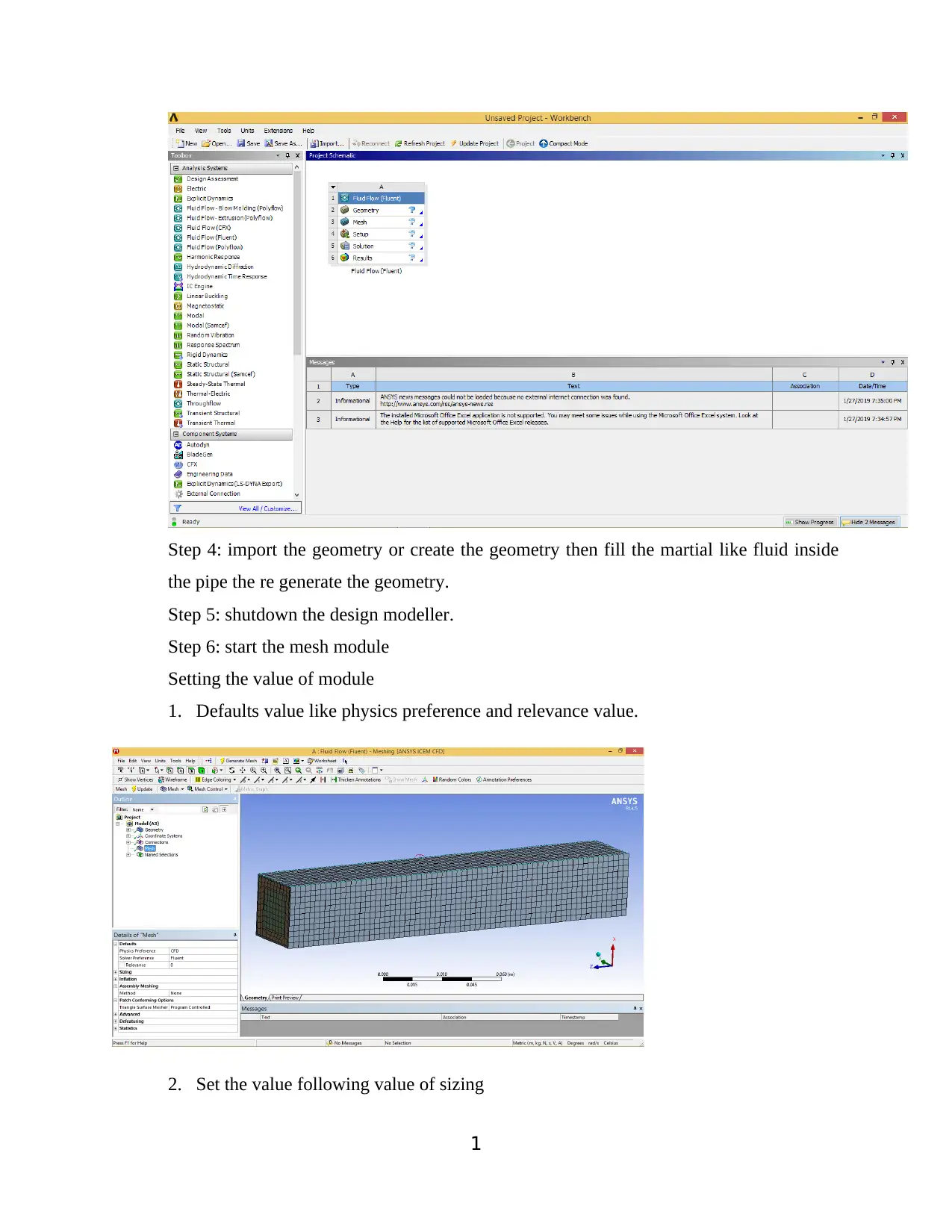
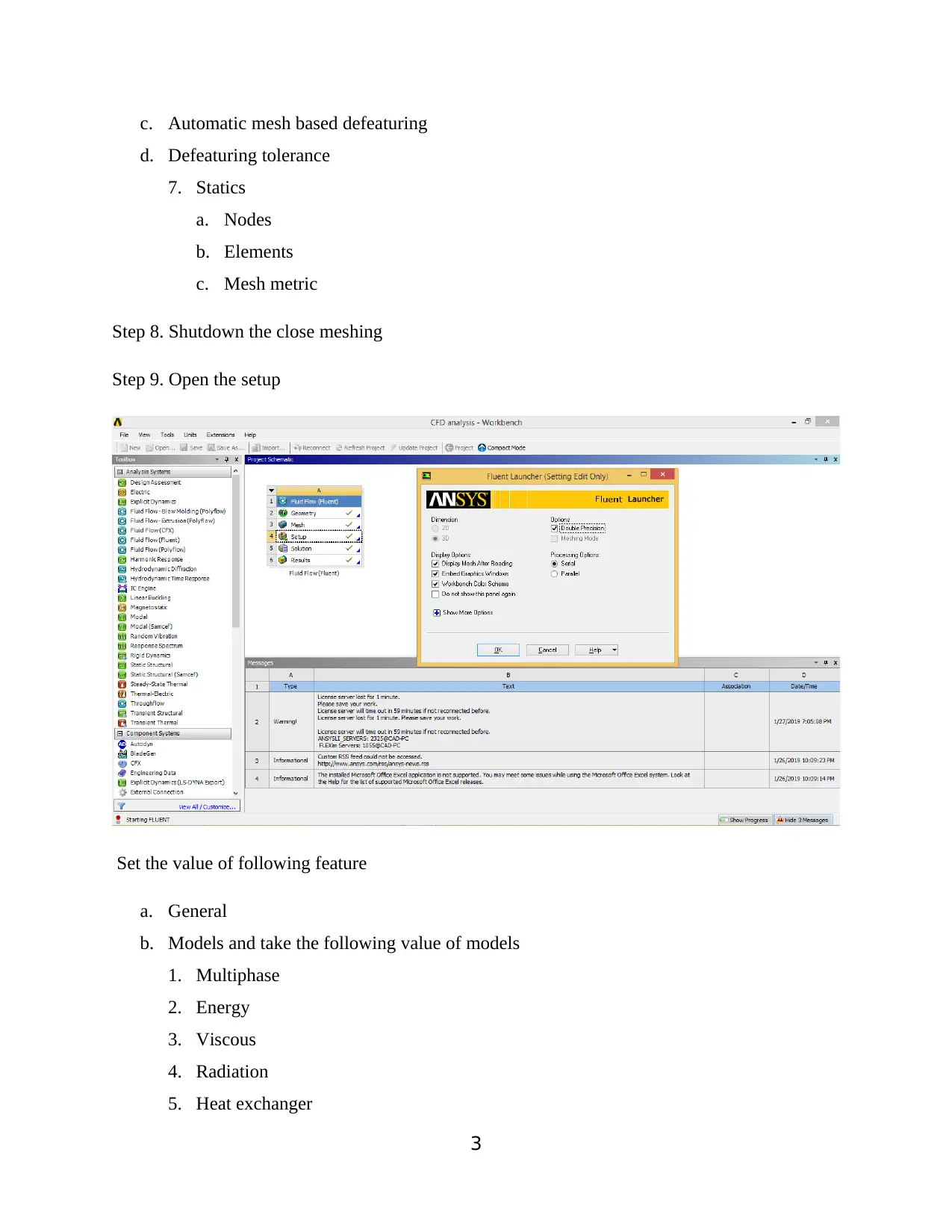
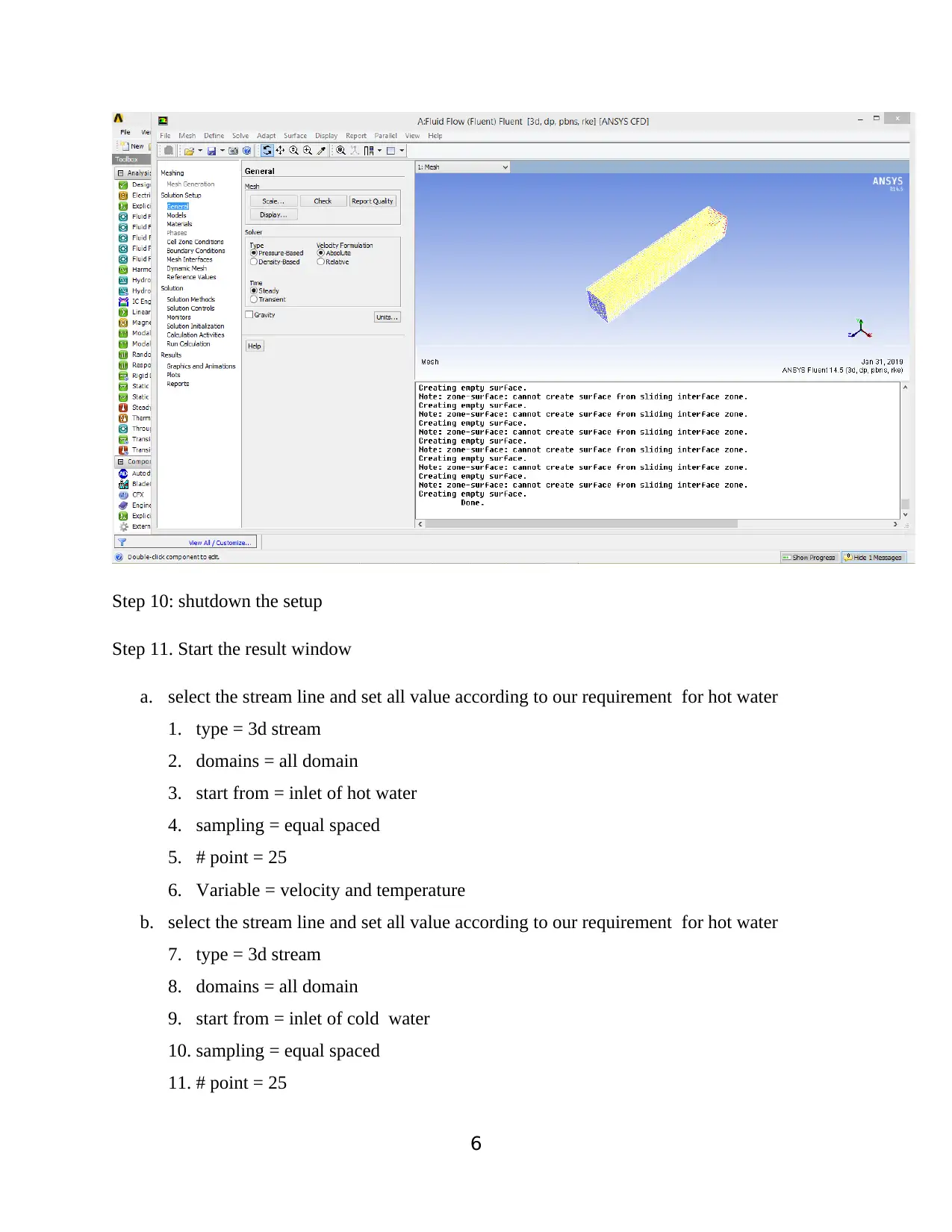
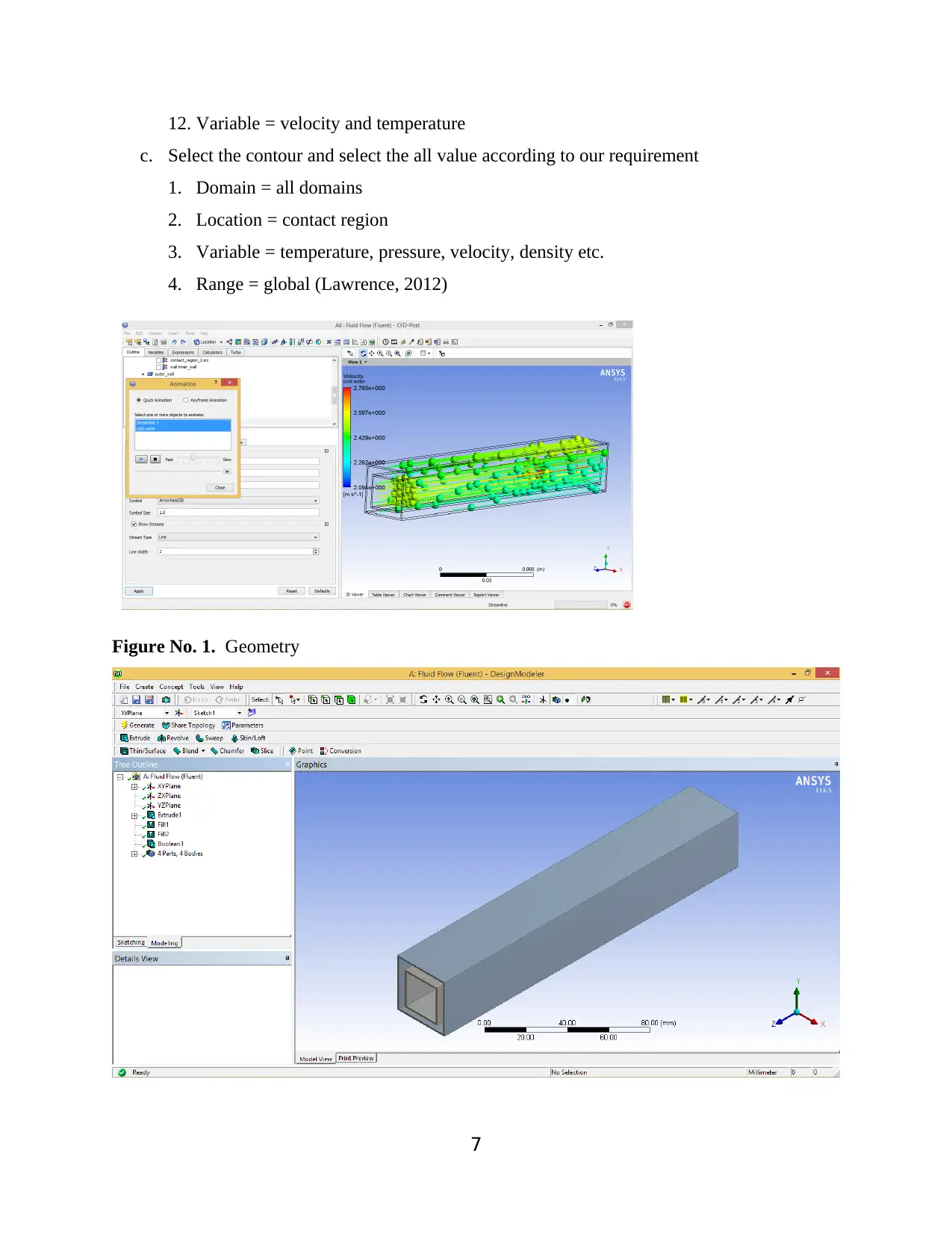
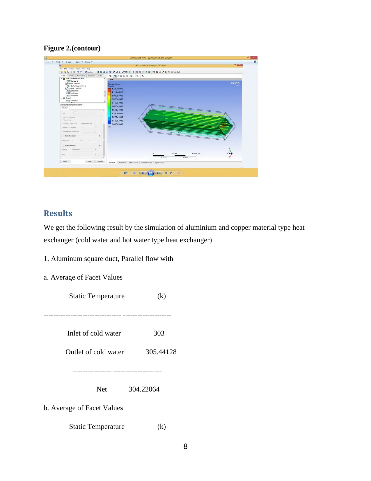
This report presents a Computational Fluid Dynamics (CFD) analysis of a heat exchanger, detailing the simulation process and results. The study involves generating a 3D model in SolidWorks, importing it into ANSYS Workbench, and utilizing the Fluid Flow (Fluent) module. The methodology includes setting up the mesh, defining material properties (water, copper, and aluminum), and applying boundary conditions such as inlet and outlet temperatures and velocities. The simulation aims to determine temperature, pressure, and velocity distributions within the heat exchanger, as well as generating streamline and contour plots. The results section compares the performance of aluminum and copper heat exchangers under parallel and counter flow configurations, reporting average temperatures at inlets and outlets. The report highlights the advantages of CFD, such as cost and time savings, and provides references to relevant literature.

CFD
[Document subtitle]
JANUARY 26, 2019
HP
[Company address]

Contents
General Information...........................................................................................................................................0
1. The objective of the simulation:- Main objective of CFD analysis is following.......................................0
Methodology......................................................................................................................................................0
Results................................................................................................................................................................8
Advantage of CFD:..........................................................................................................................................10
Disadvantage of CFD:......................................................................................................................................10
II

General Information
1. The objective of the simulation:- Main objective of CFD analysis is following
a. Find the inlet and outlet temperature of hot pipe and cold pipe and their difference.
b. Find the inlet and outlet pressure of hot pipe and cold pipe fluid and their difference.
c. Find the inlet and outlet velocity of fluid in hot pipe and cold pipe and their difference.
d. Generate the graph of stream flow of fluid
e. Generate the graph of contour flow (Munson, 2007)
Methodology
We follow the following step to analyses the heat exchanger in CFD module of ansys in work
wench.
Step1. Generate 3d model in solid works software with given dimension.
Step 2. Start workbench of ansys software.
Step3. Used fluid flow (fluent)

Step 4: import the geometry or create the geometry then fill the martial like fluid inside
the pipe the re generate the geometry.
Step 5: shutdown the design modeller.
Step 6: start the mesh module
Setting the value of module
1. Defaults value like physics preference and relevance value.
2. Set the value following value of sizing
1

a. Use advance value of size function
b. Relevance centre
c. Initial size seed
d. Smoothing
e. Span angle centre
f. Curvature normal angle
g. Min size
h. Max size
i. Growth rate
j. Minimum edge length
3. Set the inflation value
a. Use automatic inflation
b. Inflation option
c. Transition ratio
d. Maximum layers
e. Growth rate
f. Inflation algorithm
g. View advance option
4. Patch conforming options
a. Triangle surface mesher
5. Advanced
a. shape checking
b. element mid side nodes
c. straight sided element
d. number of retries
e. extra retries for assembly
f. rigid body behaviour
g. mesh morphing
6. Disfeaturing
a. Pinch tolerance
b. Generate pinch of reference
2

c. Automatic mesh based defeaturing
d. Defeaturing tolerance
7. Statics
a. Nodes
b. Elements
c. Mesh metric
Step 8. Shutdown the close meshing
Step 9. Open the setup
Set the value of following feature
a. General
b. Models and take the following value of models
1. Multiphase
2. Energy
3. Viscous
4. Radiation
5. Heat exchanger
3

6. Specie
7. Discrete phase
8. Solidification and melting
9. Acoustics
10. Eulerian wall film
c. Material – assign the following material according to our requirement.
1. Fluid – water – liquid select
2. Solid- copper and aluminium
d. Cell zone condition – assign the material of pipe and water according to our requirement
and assignment temperature also
Like. Temperature of inlet hot water = 423 kelvin
Temperature of inlet cold water = 303 kelvin
Material of pipe – aluminium & copper chose according to our requirement.
e. Set the boundary condition
1. Inlet hot water
2. Outlet hot water
3. Inlet wall
4. Outlet wall
f. Mesh interface
g. Dynamic mesh
h. Reference value
Step. 10 solution
1. Solution method
Take the value
Scheme = simple
Spatial discretization
Gradient = least square cell based
Pressure = standard
Momentum = second order upwind
Turbulent kinetic energy = first order upwind
Turbulent dissipation rate = first order upwind
4

2. Solution controls
Pressure = 0.3
Density = 1
Body force = 1
Momentum = 0.7
Turbulent kinetic energy =0.8
3. Monitors
4. Solution initialization
a. Initialization method = standard initialization
b. Compute from = inlet
c. Reference frame = relative to cell zone
d. Gauge pressure (Pascal) = 0
e. X velocity = 0
f. y velocity = 0
g. z velocity = 0
h. turbulent kinetic energy = 0.02261741
i. turbulent dissipation rate = 4.58894
Then initialize
j. run calculation
Number of iteration = 28, reporting interval = 1 and profile updated interval = 1
the calculate (G., 2017)
5

Step 10: shutdown the setup
Step 11. Start the result window
a. select the stream line and set all value according to our requirement for hot water
1. type = 3d stream
2. domains = all domain
3. start from = inlet of hot water
4. sampling = equal spaced
5. # point = 25
6. Variable = velocity and temperature
b. select the stream line and set all value according to our requirement for hot water
7. type = 3d stream
8. domains = all domain
9. start from = inlet of cold water
10. sampling = equal spaced
11. # point = 25
6

12. Variable = velocity and temperature
c. Select the contour and select the all value according to our requirement
1. Domain = all domains
2. Location = contact region
3. Variable = temperature, pressure, velocity, density etc.
4. Range = global (Lawrence, 2012)
Figure No. 1. Geometry
7

Figure 2.(contour)
Results
We get the following result by the simulation of aluminium and copper material type heat
exchanger (cold water and hot water type heat exchanger)
1. Aluminum square duct, Parallel flow with
a. Average of Facet Values
Static Temperature (k)
-------------------------------- --------------------
Inlet of cold water 303
Outlet of cold water 305.44128
---------------- --------------------
Net 304.22064
b. Average of Facet Values
Static Temperature (k)
8

-------------------------------- --------------------
Inlet of hot water 423
Outlet of hot water 420.47504
---------------- --------------------
Net 421.73752
2. Copper square duct, Parallel flow with
a. Average of Facet Values
Static Temperature (k)
-------------------------------- --------------------
Inlet of cold water 303
Outlet of cold water 305.4761
---------------- --------------------
Net 304.23804
b. Average of Facet Values
Static Temperature (k)
-------------------------------- --------------------
Inlet of hot water 423
Outlet of hot water 420.44254
---------------- --------------------
Net 421.72128
3. Copper square duct, Counter flow with
a. Average of Facet Values
Static Temperature (k)
-------------------------------- --------------------
Inlet cold water 303
Outlet cold water 305.491
9