CFD Analysis of Fin Configuration for Heat Transfer - Unit 301023

This report presents a Computational Fluid Dynamics (CFD) analysis, focusing on heat transfer problems solved using ANSYS Fluent. It includes an introduction to CFD, its applications, advantages, and disadvantages, along with a detailed methodology for simulating fluid flow and heat transfer in a given box. The report covers discretization methods like Finite Element Method (FEM) and Finite Volume Method (FVM), spectral methods, and the governing equations of fluid dynamics, including conservation of mass, Newton's second law, and conservation of energy. It also discusses flow lines, acceleration in fluid motion, iso-surfaces, contours, circulation, and vorticity. The aim of the simulation is to create a computational model of a box to analyze its behavior, with steps outlined from workbench setup to post-processing and data analysis. The assignment brief involves determining the best fin configuration for heat dissipation using ANSYS Fluent, emphasizing the importance of avoiding plagiarism and submitting the report on time.

CFD
[Document subtitle]
[DATE]
[Company name]
[Company address]

Table of Contents
1. Objective of simulation.
2. Introduction to CFD.
3. Introduction of CFD in fluid dynamics.
4. Aim of the simulation
5. Applications of CFD
6. Advantages of CFD
7. Disadvantages of CFD
8. Future of CFD
I

General Information
1. Objective of the simulation:- Computational Fluid dynamics analysis of a given box.
Introduction:- In recent years we have seen a rapid increase in the use of computers for engineers in
solving the problems. In the same contrast particularly Computational Fluid Dynamics (CFD) is true
subject for the problem solving that involves fluid heat transfer and fluid flow which occur in
applications related aerospace, power sector and automobile industry. The various factors that are the
reasons for the development of CFD are:-
 Growth in the complexity of the engineering problems that can be unsolved in manual
way.
 Need of quick solution with moderate accuracy.
 The expenses that an industry bears during laboratory experiment of physical prototype.
 The absence of analytical solutions.
 Exponential growth in the number crunching abilities and rigorous computer speed and
its memory.[1]
2. Introduction to CFD:-
Question: What is CFD?
CFD is a method adopted to obtain a discrete solution of problems related to fluid in a
real world. The discrete solution is a solution obtained by a finite collection of space
points and the level of discrete time. CFD is physical quality of any fluid - flow that is
having three governing fundamental principles:-
 Conservation of mass for the fluid.
 Newton’s Second Law :- Which say-s that the rate of the change of momentum is
directly pro-portional to the force applied and this rate of change of moment-um
is directly proportional to the applied force and in the direction of the applied
force.
 Law of conservation of energy which is the first law of thermodynamics and it
states that the summation of the rate of change of heat addition must be equal to
the work done on the fluid.
In order to continue the understanding of CFD the person must first understand the fluid dynamics and
its governing equation.
2

The Computational Fluid Dynamics equations can be derived in two stages.
 First stage is the numerical discretization.
 Second stage is the specific technique.
The above two stages are used to solve the algebraic equations which is derived
from the governing equations.
2.1. Discretization: - The discretization process are identified by
some common methods that we are still using today. The two most
common methods are the finite-element and spectral methods.
2.1.1. Finite Element Method
The finite element method is an oldest method among all methods in solving the
numerical solution of partial differential equations. This method was derived by
Euler in year 1768. It is used to get numerical solutions of the differential equations
by manual calculation i.e. by hand calculation. In this method at a number of
grids/elements are defined with their respective nodal points. Each grid with the
number of nodal points are use-d to describe the fluid - flow domain. Then the
concept of Taylor series expansion is applied in-order to generate finite-difference
approximation-s to the partial derivatives of the governing equations. These
derivatives are then replaced by using finite-difference approximations and this all
results in an algebraic equation for the flow solution at each of the grid point. This
method is most commonly used in structured grids since it requires a mesh having
a high degree of regularity and accuracy. From all above discussion Finite Element
Method can be summarized in three basic features:-
1. Bifurcate the whole body / structure into parts, finite element.
2. For each representative elements create the relations among
secondary and primary variable.
3. Assemble of the elements to obtain the relations in form of equation or
a matrix between the secondary and primary variables.
As per discretization is concerned the two compatibility conditions must be
ensured:-
1. Compatibility of nodal displacement:- When a body is deformed
without breaking, no crack appears in stretching and particles do not
penetrates each other in elements. Such situation is called Nodal
3

displacement compatibility. The compatibility condition confirms that
the displacement is continuous and single value function of position.
2. Equilibrium of forces:- The equilibrium at the nodal forces must be
ensured.
Although there are a numerous of commercial and research codes that are
available and they can be employed but the in finite-element method CFD
application is not so much fruitful. But apart from this there is one method which
is in brief same as finite element method and is seems fruitful and commercially
uses all codes and is essentially used by CFD. The method is called “Finite -
Volume Method (FVM)”. The only differentiating feature is that FVM uses simple
piecewise polynomial functions for local elements which tends to describe the
variations of the un-known flow variables. The weighted residual concept is
introduced in order to evaluate the errors associated with the approximate
functions, which are later surely minimized. A set of non-linear algebraic
equations for the unknown terms of the approximating functions is solved, hence
resulting in the flow solution. The residual functions are solved and the flow
solutions are obtained by, Collocation method, Galerkins method, Sub-domain
method, and least square method.
2.1.2. Spectral method
Spectral method has a same general approach as that of the finite-difference
and finite-element methods, where the unknowns of the equations that are
governed are replaced with a some short series. The difference is in only the
methods of implementation. The previous two methods uses local
approximations but the spectral method implements global approximation. That
is by means of Fourier series, Legendre polynomials, for the entire flow body /
domain. The conflict between the exact solution and the approximate solution is
dealt with by the use of a weighted residuals concept similar to the finite-
element method.
The instrument which has allows the practical growth of CFD has a high speed digital computer with a
great efficiency. CFD solutions generally requires the repetitive manipulation of many thousands, even
millions of numbers, a task that is impossible for any human without the aid of a computer. Therefore,
advancement in CFD, and its applications to problems of more detail and sophistication, are intimately
related to advances in computer hardware, particularly in regard to storage and execution speed. This is
why the strongest force driving the development of new supercomputer is coming from CFD
community.
Steps in CFD Analysis
1. Getting the real world flow problems
2. Mathematical modelling of the given body which includes the general equations,
boundary conditions etc.
4

3. Generating the discrete equations (preferably the algebraic equations).
4. Finding the solution of the above algebraic equations.
5. Post processing and the data analysis and finally the flow visualization.
3. Introduction of CFD in fluid dynamics
Study of motion of the fluid with reference of forces and moments is known as fluid dynamics. In fluid
flow there different types of forces occurs in the flow like viscous forces, gravitational forces, pressure
forces, surface tension forces, eddy forces (turbulent forces) and different type of other forces.
All CFD in one form is based on governing equations of fluid dynamics- the continuity equation,
momentum equations and energy equations. These equations speak the physics. Basically the equations
are the mathematical statements of three fundamental physical principles upon which all of the fluid
dynamics is based upon:
 Conservation of mass.
 Newton’s second law i.e. F=ma.
 Conservation of energy.
 During the vehicle in motion when the fluid flows under adverse
pressure condition, fluid loses its momentum. Near the surface the
particles have less momentum so they looses their momentum fastly.
At the point where momentum of the fluid becomes zero and after
which near the surface the fluid surface the fluid moves under adverse
pressure condition i.e. in reverse direction that point is known as point
of separation. It is not compulsory that separation must be present in
adverse pressure condition.
In fluid flow velocity is function of space and time, so the acceleration is the function of
space and time. Space component is known as convective acceleration and time
component is known as local acceleration. During the ANSYS analysis the above
acceleration place an important role and help the engineer to make proper aerodynamic
design of the vehicle. This is so because the acceleration and velocity component are
responsible for lift and drag of the vehicle. Improper design leads to create serious lift of
vehicle and this may results in serious accident. Inorder to avoid this impact in the
absence of physical prototype graphically the prototype is designed and is tested through
computer itself by the use of ANSYS and employing Computational Fluid Dynamics
theory.
5

Apart from the above concept some terms need to be described which will helps to validate the whole
analysis:-
1. Flow Lines:- Fluid flow can be described by 3 flow lines
 Stream line:- It is an imaginary line or curve drawn in space such that tangent
drawn gives velocity vector i.e. velocity vector and stream line vector coincides.
The two streamlines never intersect each other as well as stream line also never
intersects itself because at the point of intersection there will be two velocity
fields which is impossible. So there is no flow across the streamlines.
 Path line:- The line drawn by tracing the path of single fluid particle at different
time integrals. It is defined on the basis of ‘Langrangian description’.
 Streak line:- It is an instantaneous picture of all fluid particles passing through
single point.
NOTE:- For the steady flow all three lines are identical i.e. all three line coincides.
2. Acceleration in fluid motion:- The velocity is the function of time and spacde in the fluid
flow, so the acceleration is the function of space and time. Space component is known as
convective acceleration and time component is known as Local acceleration.
3. Iso-surface:- An iso-surface is a 3D isoline. It is a type of surface
representing the points of a constant value (e.g. pressure,
temperature, velocity, density) which is within a volume of space; in
other words, it is that level set of a continuous function whose domain
is 3D-space. It is a surface which is defined by an implicit equation.
i.e. F (x,y,z) = f
where, F is the function of space and f is the constant.
The `Iso-surface' is a representation that is used to compute and draw a surface within a volumetric
data field on a 3-D surface corresponding to points with a single scalar value. It is displayed by data
set, iso-value, draw (Points, Shaded Points, Wireframe, or Solid Surface), boundary, step and size. It
is normally displayed by computer graphics. It used as data visualization methods
in computational fluid dynamics (CFD) that helps the engineers to study the
features of fluid flow. It is mostly helpful in design the system related to
aerodynamics such as aircraft wings or the super cars models.
4. Contours:- It is an outline representing or bounding the shape or form of
something. It is used for representation of typical response system in
6

other words we can say it is typical curve line which describes the
response system.
5. Circulation:- It is the line integration of tangential component of
velocity along the closed loop. It is the scalar quantity.
6. Vorticity:- It is the mathematical measure of rotationality. It is circulation per unit area. It
is wice of the rotation. The direction of vorticity is as that of rotation.
4. Aim of the simulation
To create a computational model of the given box in order to do analyse the box showing its behaviour. .
5. Methodology Adopted
Step1: start the workbench window in system
Step2: select the fluid flow fluent on ansys window.
1. Design assessment
2. Electric
3. Explicitly dynamics
4. Fluid flow – blow molding (polyflow)
5. Fluid flow – blow extrusion (polyflow)
6. Fluid flow(CFX)
7. Fluid flow (fluent)
8. Fluid flow (polyflow)
9. Harmonic response
10. Hydrodynamic diffraction.
7

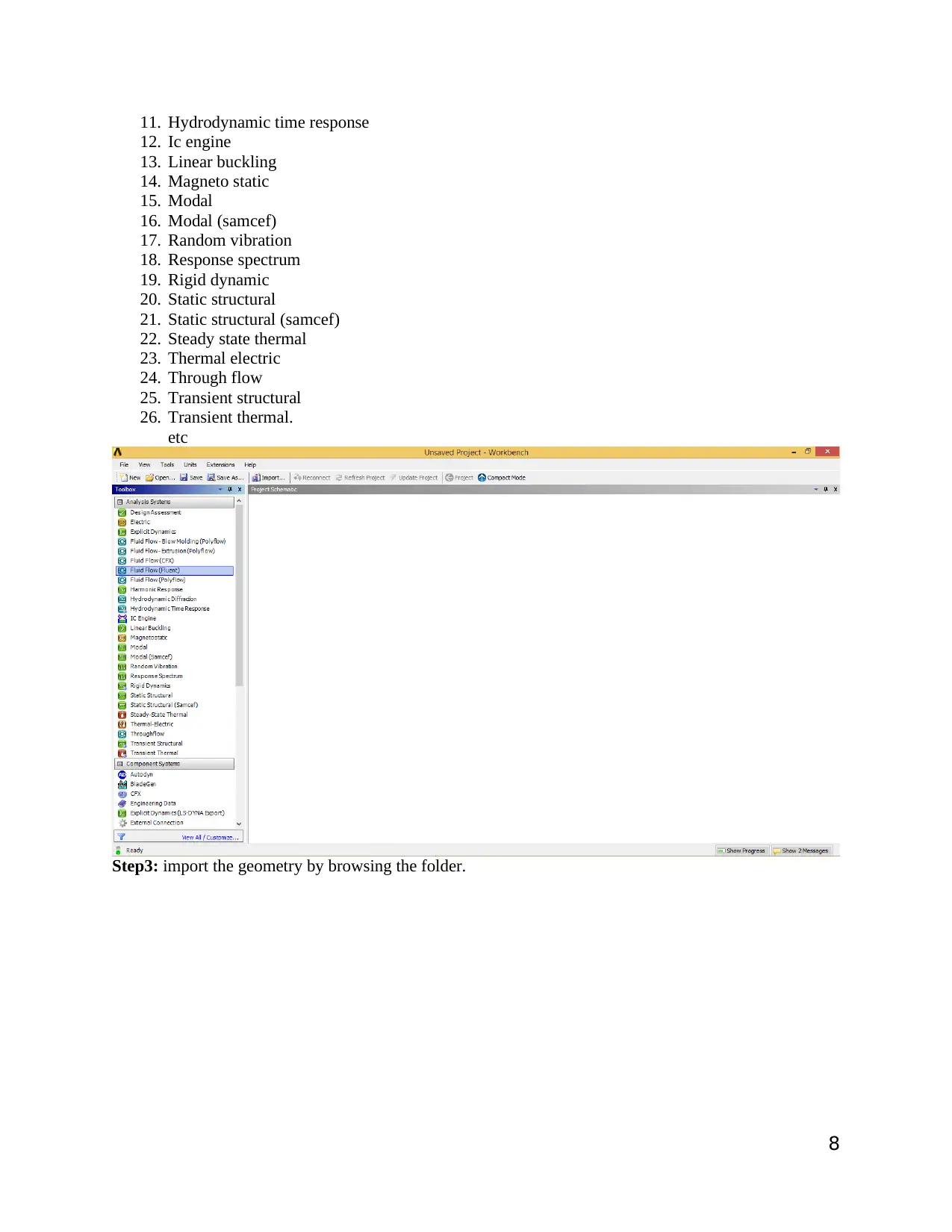
11. Hydrodynamic time response
12. Ic engine
13. Linear buckling
14. Magneto static
15. Modal
16. Modal (samcef)
17. Random vibration
18. Response spectrum
19. Rigid dynamic
20. Static structural
21. Static structural (samcef)
22. Steady state thermal
23. Thermal electric
24. Through flow
25. Transient structural
26. Transient thermal.
etc
Step3: import the geometry by browsing the folder.
8

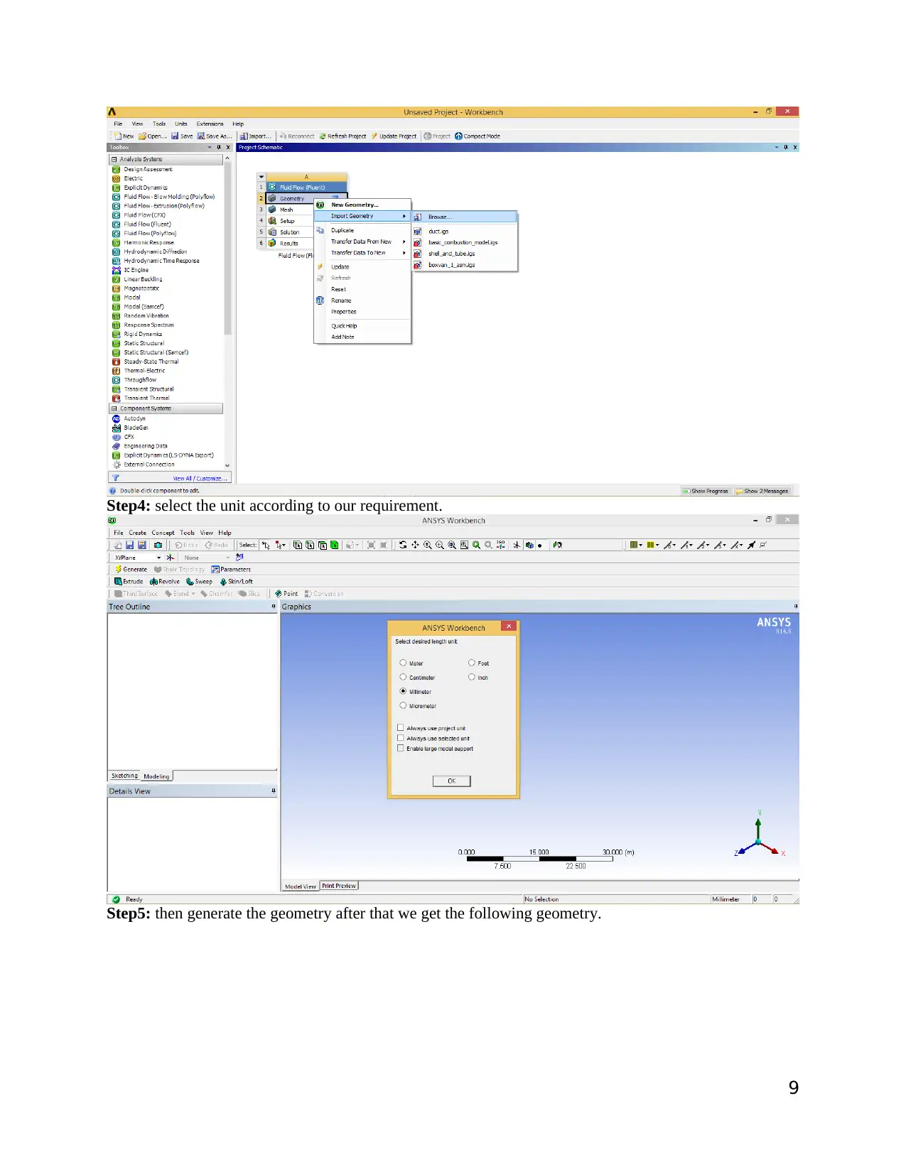
Step4: select the unit according to our requirement.
Step5: then generate the geometry after that we get the following geometry.
9

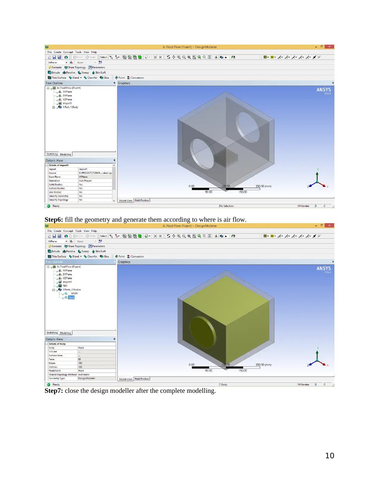
Step6: fill the geometry and generate them according to where is air flow.
Step7: close the design modeller after the complete modelling.
10

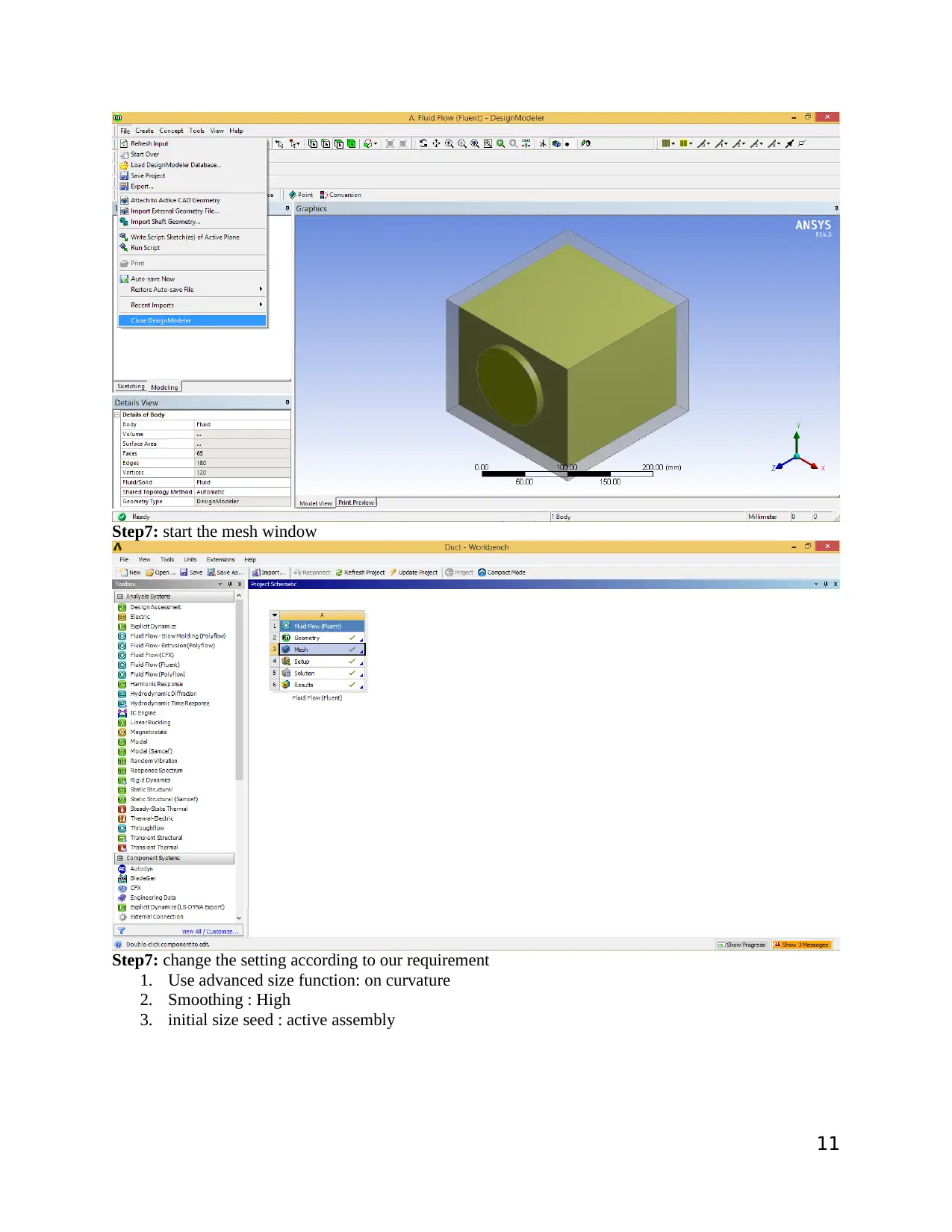
Step7: start the mesh window
Step7: change the setting according to our requirement
1. Use advanced size function: on curvature
2. Smoothing : High
3. initial size seed : active assembly
11

Step8: Generate the mesh according to our requirement.
Step9: close the meshing window
12

Step10: open the setup file on window
Step10: then select on the double precision on window
13

Step11: select the models then select the energy question
Step12: then select the viscous then select the k-epsilon (2eqn) then select the realizable then select the
enhanced wall treatment.
14

Step12: then select the material of fluid as air
Step13: then select the material of solid as aluminium.
15

Step13: then select the cell zone condition fluid as an air and wall as a solid
Step13: then select the boundary condition
16

Step13: then select the boundary condition inlet fluid then mass flow inlet then thermal condition and fill
the total inlet temperature 293
Step14: then select the solution methods then scheme as simple and gradient as least squares cell based
and pressure and momentum as second order upwind and turbulence kinetic energy and turbulence kinetic
energy as first order upwind and turbulence dissipation rate as first order upwind.
17

Step13: then select the condition control then put the value pressure, density, body forces, momentum
and turbulence kinetic energy.
Step13: then select the monitors then select residuals, print, and plot. And statics off
18

Step14: then select the solution initialization then select standard initialization and select compute from
all zones and reference from as relative to cell zone and give the initial values.
Gauge pressure (Pascal) x velocity (m/s) , y velocity (m/s), ) z velocity (m/s), turbulence kinetic energy
(m^2/s^2) and turbulence dissipation rate(m^2/s^3) then initialize and it take the some time.
Step15: then select the run calculation then put the value of number of iterations 50, reporting interval 1
and profile update interval 1 then calculate.
19

Step16: then close the window.
Step16: then select the solution window
20

Step16: then select the solution window
Step17: then select the graphics and animation, and graphics, mesh, contours, vectors, path line and
practical tracks tracks and sweep surface, scene animation, solution animation.
21

Step17: then close fluent.
Step18: then select the results
22

Step18: then select the stream line then type 3D stream line, domains all domains, and start from inlet
fluid and sampling equally spaced and # of points 25 and variable and velocity then apply.
Step18: then select the velocity contour, domains all domains, location contact region src, variable
temperature, range global and colour scale linear and colour map default (rainbow)
23

Result: select the results then select the reports surface integrals then report type facet average, field
variable temperature, static temperature inlet fluid and outlet fluid select then we get the temperature
difference in outlet and outlet fluid then compute the compute then we get the value of inlet and outlet
temperature. According to our requirement we select the inlet and outlet fluid, etc.
1 The fines are parallel to the x-direction.
a. The centres of the inlet and outlet ducts are 70 mm above the bottom.
Static Temperature (k)
-------------------------------- --------------------
Inlet fluid 293
Outlet fluid 293.38947
---------------- --------------------
Net 293.192
24

c. The centres of the inlet and outlet ducts are 100 mm above the bottom.
Average of Facet Values
Static Temperature (k)
-------------------------------- --------------------
Inlet air 293
Outlet air 293.30762
---------------- --------------------
Net 293.15298
1 The fines are parallel to the y-direction.
a. The centres of the inlet and outlet ducts are 70 mm above the bottom.
Average of Facet Values
Static Temperature (k)
-------------------------------- --------------------
Inlet air 293
Outlet air 293.00143
---------------- --------------------
Net 293.0007
25

c. The centres of the inlet and outlet ducts are 100 mm above the bottom.
Average of Facet Values
Average of Facet Values
Static Temperature (k)
-------------------------------- --------------------
Inlet air 293
Outlet air 293.32932
---------------- --------------------
Net 293.16983
Conclusion: According to above result we found lowest temperature on fin when The centres of the
inlet and outlet ducts are 70 mm above the bottom.
26

Applications of CFD:-
1. Aerospace industries.
2. Automobiles.
3. Biomedical
4. Chemical processing.
5. Marines
6. Oil and gas piping industries.
7. Sports etc.
Advantages of CFD
1. Eliminates the process of experimentation in laborartories.
2. Provides better details.
3. Provides better predictions in a short peroids of time.
4. Provides better and fast design meeting all the environmental regulations and ensures
industry quality.
5. Provides shorter design cycles and supply products faster in the market.
6. Easy to install with minimum downtime.
7. Allows rapid prototyping.
27

8. More cost effective.
6. Disadvantages of CFD
1. Initial investment cost is high.
2. Required skilled persons therefore costly in field of professionals.
7. Future of CFD
After the above analysis we have reached a certain platform in understanding of and appreciation for
CFD. CFD is the new “third dimension” in fluid dynamics, equally sharing the stage with the other
dimension of pure theory and pure experiment.
CFD has already had a major impact on car design, and had became the critical technology for
aerodynamic design over the next decade. There is no doubt that a major focus of CFD is to enhance the
design process for any machine that deals with fluid.
Today, CFD is used to calculate complete three dimensional flow fields over real cars.
The major role of CFD is that of research, a tool to enhance our undersytanding of the basic physical
nature of fluid dynamics.
References
There are no sources in the current document.
1. Review: CFD Applications in the Automotive Industry. M. N.
Dhaubhadel J. Fluids Eng 118(4), 647-653 (Dec 01, 1996) (7
pages)doi:10.1115/1.2835492History: Received March 28, 1996;
Revised July 18, 1996; Online January 22, 2008.
2. Book:- Computational Fluid Dynamics- The basics with applications.
John D. Anderson, Jr. Dept. Of Aerospace Engineering University of
Maryland.
3. Automotive computational fluid dynamics simulation of a car using
ANSYS. Praveen Padagannavar and Manohara Bheemanna School of
Aerospace, Mechanical & Manufacturing Engineering Royal Melbourne
Institute of Technology (RMIT University) Melbourne, VIC 3001,
Australia
28

4. Janvijay Pateriya, Raj Kumar Yadav, Vikas Mukhraiya and Pankaj Singh,
Brake Disc Analysis with the Help of Ansys Software. International
Journal of Mechanical Engineering and Technology, 6(11), 2015, pp.
114–122.
5. Rakesh Jaiswal, Anupam Raj Jha, Anush Karki, Debayan Das, Pawan
Jaiswal, Saurav Rajgadia, Ankit Basnet and Rabindra Nath Barman,
Structural and Thermal Analysis of Disc Brake Using Solidworks and
Ansys. International Journal of Mechanical Engineering and Technology,
7(1), 2016, pp. 67–77.
6. Anderson, ‘Race Car Aerodynamics Part 2: Lift and Drag’, 2014.
7. J.Ducoste, ‘An Overview of Computational Fluid Dynamics’, 2008
8. Katz, J. 1995, ‘Race car aerodynamics: Designing for speed’, 1st edn,
Robert Bentley.
9. Mampeay, F., and Z. A.Xu “An experimental and simulation Study of
mold filling combined with heat transfer”. In C. Hirsch, J, Periaux and
W. Kordulla(eds.), Computational Fluid dynamics ’92, vol. 1, Elsevier,
Amsterdam,1992,pp. 421-428.
29