Real World Analytics: Heating/Cooling Load Analysis, Data Analysis
VerifiedAdded on 2021/06/17
|15
|1161
|15
Project
AI Summary
This project analyzes heating and cooling loads in buildings, focusing on variables like relative compactness, surface area, wall area, roof area, and overall height. The analysis uses a dataset of 300 samples and is conducted in R software. Task 1 involves data visualization using histograms and scatterplots to understand the distribution and correlation of variables. Task 2 identifies and removes an insignificant variable (X3). Task 3 calculates weighted means and power means, comparing different models for error measures and correlations. Task 4 presents a linear regression model, highlighting the relationships between the dependent variable (heating load) and the independent variables. The project provides insights into energy-efficient building design and optimization of energy consumption.

Running head: REAL WORLD ANALYTICS
Real World Analytics
Name of Student:
Name of University:
Author’s Note:
Real World Analytics
Name of Student:
Name of University:
Author’s Note:
Paraphrase This Document
Need a fresh take? Get an instant paraphrase of this document with our AI Paraphraser
1REAL WORLD ANALYTICS
Part A:
Description:
The concepts of “heating load” and “cooling load” are utilized to help in understanding
the specifications of the equipment for the purposes of heating and cooling in the buildings
where they are applicable. Thus it can be said that these are major variables which are to be kept
in mind at the time of the creation and design of energy efficient buildings at the time of
considering the ways in which the energy consumption can be optimized. There are two specific
variables which are to be considered in this assignment. The variables which are considered are
that of Heating Load (Y1 or HL) and Cooling Load (Y2 or CL).
The two variables which are to be considered are the heating and cooling load. The
independent variable which are to be considered are relative compactness (X1), which is
considered in percentage, the surface area (X2) which is considered in square meters, the wall
area (X3) is considered in square meter, the area of the roof (X4) considered in square meter and
finally the overall height (X5) are to be considered as potential influences on the response which
has been considered. Out of a total of 700-800 points, a random sample of 300 has been chosen
for the analysis. The analysis was conducted in the R software.
Task 1:
The required data file is downloaded from the CloudDeakin website that has been
maintained as per the instructions. In this case the dependent variable is that of the “heating
load” is considered to be the variable of interest and it is also the dependent variable. The
2REAL WORLD ANALYTICS
independent variables, dependent variables, the graphical and visual representations and the
histogram plots indicate the distribution of the variables.
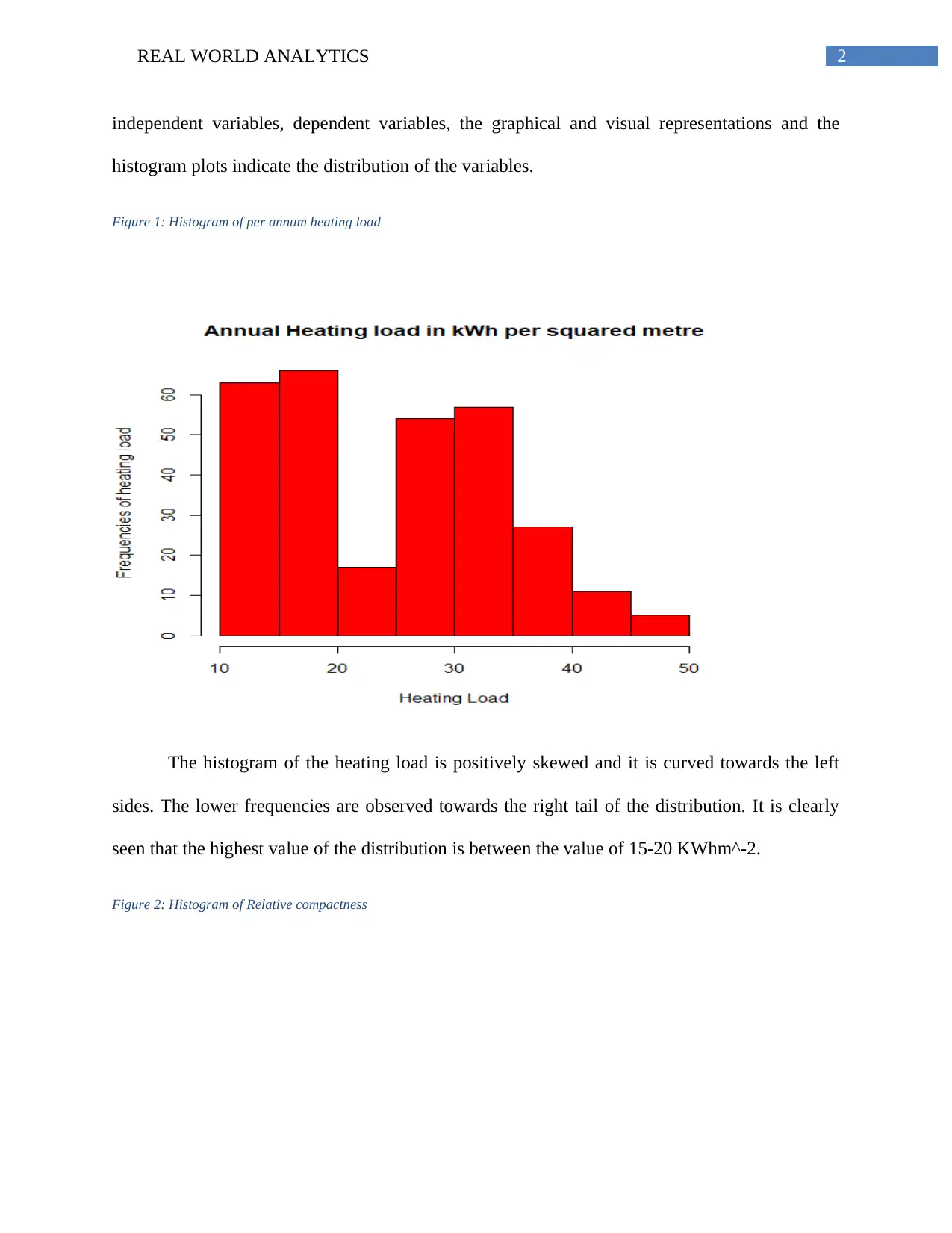
Figure 1: Histogram of per annum heating load
The histogram of the heating load is positively skewed and it is curved towards the left
sides. The lower frequencies are observed towards the right tail of the distribution. It is clearly
seen that the highest value of the distribution is between the value of 15-20 KWhm^-2.
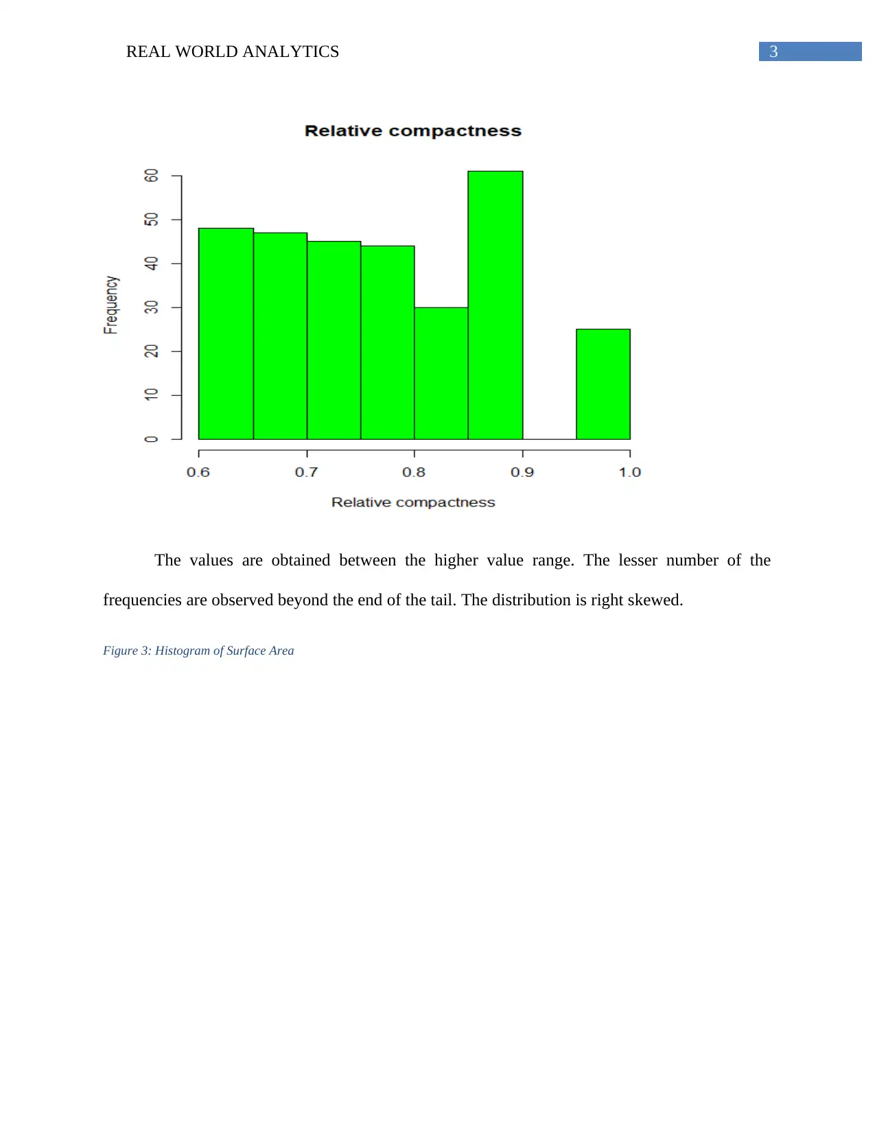
Figure 2: Histogram of Relative compactness
⊘ This is a preview!⊘
Do you want full access?
Subscribe today to unlock all pages.

Trusted by 1+ million students worldwide
3REAL WORLD ANALYTICS
The values are obtained between the higher value range. The lesser number of the
frequencies are observed beyond the end of the tail. The distribution is right skewed.
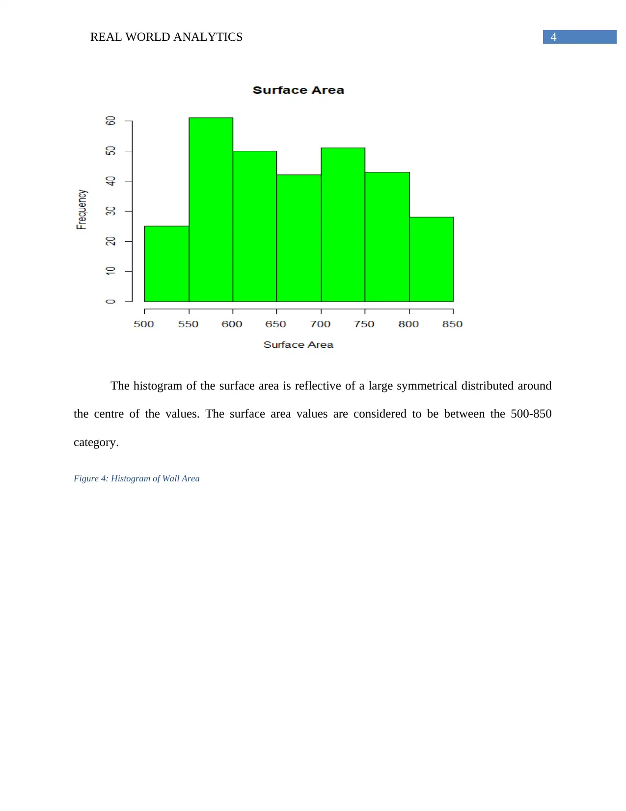
Figure 3: Histogram of Surface Area
The values are obtained between the higher value range. The lesser number of the
frequencies are observed beyond the end of the tail. The distribution is right skewed.
Figure 3: Histogram of Surface Area
Paraphrase This Document
Need a fresh take? Get an instant paraphrase of this document with our AI Paraphraser
4REAL WORLD ANALYTICS
The histogram of the surface area is reflective of a large symmetrical distributed around
the centre of the values. The surface area values are considered to be between the 500-850
category.
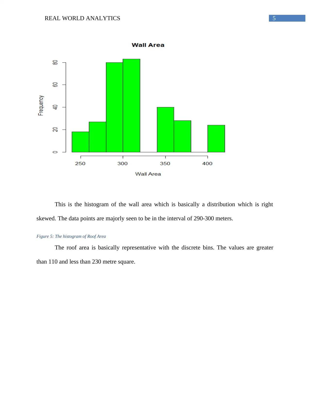
Figure 4: Histogram of Wall Area
The histogram of the surface area is reflective of a large symmetrical distributed around
the centre of the values. The surface area values are considered to be between the 500-850
category.
Figure 4: Histogram of Wall Area
5REAL WORLD ANALYTICS
This is the histogram of the wall area which is basically a distribution which is right
skewed. The data points are majorly seen to be in the interval of 290-300 meters.
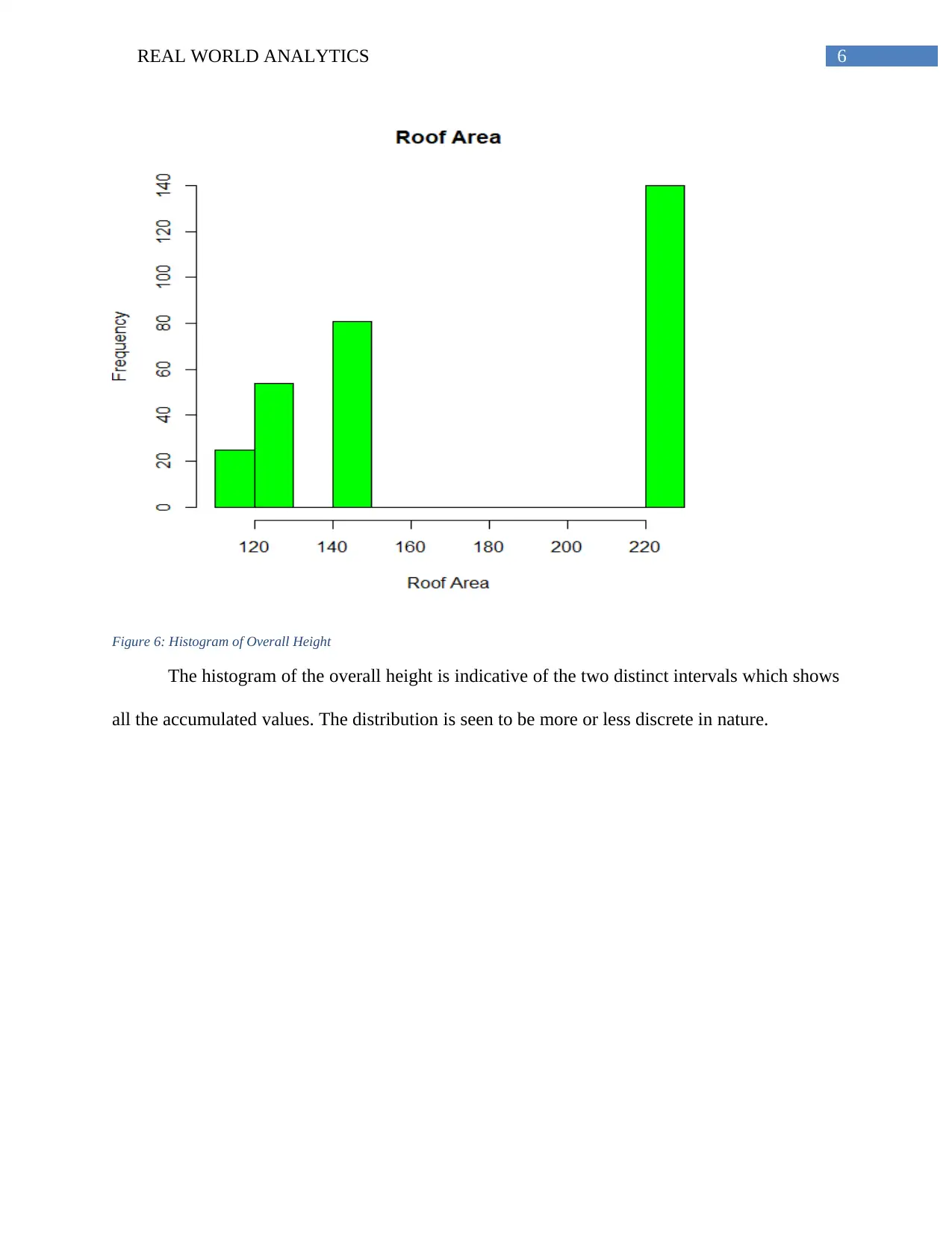
Figure 5: The histogram of Roof Area
The roof area is basically representative with the discrete bins. The values are greater
than 110 and less than 230 metre square.
⊘ This is a preview!⊘
Do you want full access?
Subscribe today to unlock all pages.

Trusted by 1+ million students worldwide
6REAL WORLD ANALYTICS
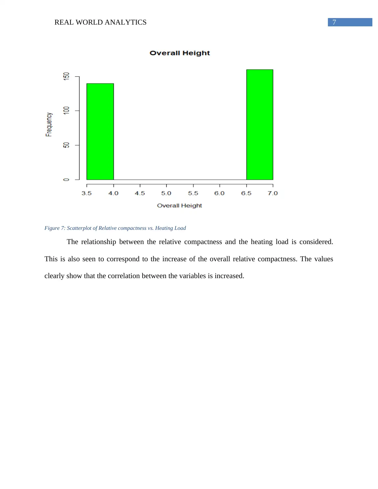
Figure 6: Histogram of Overall Height
The histogram of the overall height is indicative of the two distinct intervals which shows
all the accumulated values. The distribution is seen to be more or less discrete in nature.
Figure 6: Histogram of Overall Height
The histogram of the overall height is indicative of the two distinct intervals which shows
all the accumulated values. The distribution is seen to be more or less discrete in nature.
Paraphrase This Document
Need a fresh take? Get an instant paraphrase of this document with our AI Paraphraser
7REAL WORLD ANALYTICS
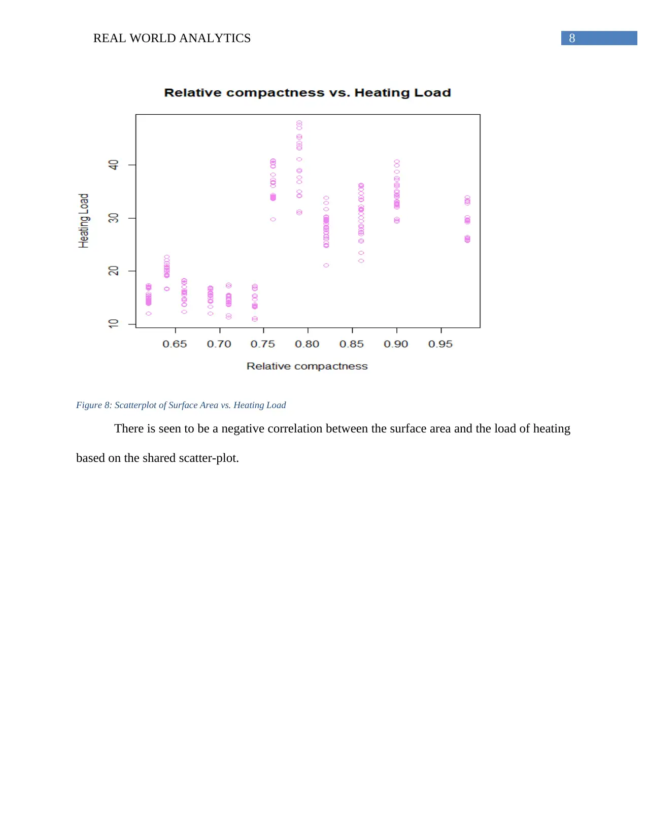
Figure 7: Scatterplot of Relative compactness vs. Heating Load
The relationship between the relative compactness and the heating load is considered.
This is also seen to correspond to the increase of the overall relative compactness. The values
clearly show that the correlation between the variables is increased.
8REAL WORLD ANALYTICS
Figure 8: Scatterplot of Surface Area vs. Heating Load
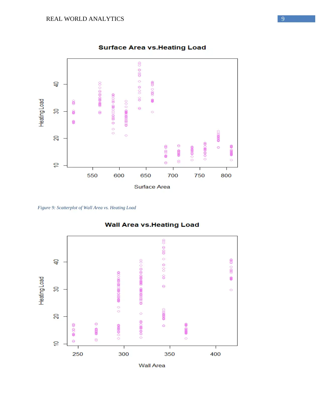
There is seen to be a negative correlation between the surface area and the load of heating
based on the shared scatter-plot.
Figure 8: Scatterplot of Surface Area vs. Heating Load
There is seen to be a negative correlation between the surface area and the load of heating
based on the shared scatter-plot.
⊘ This is a preview!⊘
Do you want full access?
Subscribe today to unlock all pages.

Trusted by 1+ million students worldwide
9REAL WORLD ANALYTICS
Figure 9: Scatterplot of Wall Area vs. Heating Load
Figure 9: Scatterplot of Wall Area vs. Heating Load
Paraphrase This Document
Need a fresh take? Get an instant paraphrase of this document with our AI Paraphraser
10REAL WORLD ANALYTICS
The histogram is clearly indicative of the fact that the wall area and the heating load as
variables are associated with a moderate and positive degree of association.
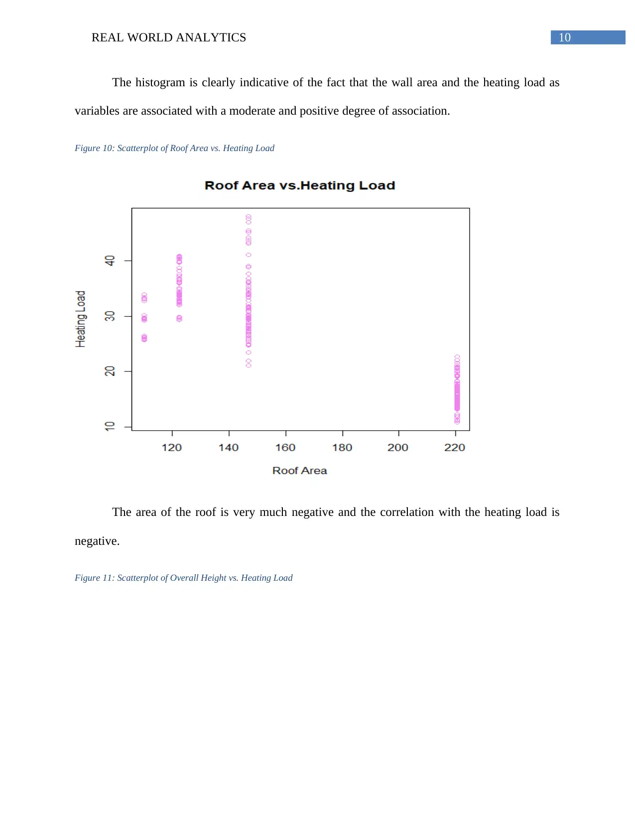
Figure 10: Scatterplot of Roof Area vs. Heating Load
The area of the roof is very much negative and the correlation with the heating load is
negative.
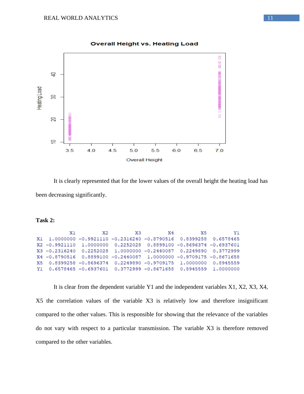
Figure 11: Scatterplot of Overall Height vs. Heating Load
11REAL WORLD ANALYTICS
It is clearly represented that for the lower values of the overall height the heating load has
been decreasing significantly.
Task 2:
It is clear from the dependent variable Y1 and the independent variables X1, X2, X3, X4,
X5 the correlation values of the variable X3 is relatively low and therefore insignificant
compared to the other values. This is responsible for showing that the relevance of the variables
do not vary with respect to a particular transmission. The variable X3 is therefore removed
compared to the other variables.
⊘ This is a preview!⊘
Do you want full access?
Subscribe today to unlock all pages.

Trusted by 1+ million students worldwide
1 out of 15
Related Documents
Your All-in-One AI-Powered Toolkit for Academic Success.
+13062052269
info@desklib.com
Available 24*7 on WhatsApp / Email
![[object Object]](/_next/static/media/star-bottom.7253800d.svg)
Unlock your academic potential
Copyright © 2020–2026 A2Z Services. All Rights Reserved. Developed and managed by ZUCOL.


