PLAN60572: Hedonic Pricing Model for Aberdeen Housing Data
VerifiedAdded on 2022/12/19
|13
|4087
|1
Project
AI Summary
This assignment explores the application of a hedonic pricing model (HPM) to analyze factors affecting house prices in the real estate market. The study begins with an introduction to hedonic pricing, defining it as a model that considers both internal and external factors influencing property prices. A comprehensive literature review covers the history and applications of HPM, including its use in various research fields and its flexibility in determining the relationship between market products and external factors. The methodology section details the use of quantitative data from Aberdeen, including fourteen variables such as sale price, time on the market, dwelling type, and distances to amenities. A regression model was constructed using the backward method to determine the best predictors of house prices. The results, presented in tables, show a high degree of correlation between variables and the model's ability to explain the dependent variable (sale price). The ANOVA and coefficients tables further analyze the statistical significance and the impact of individual variables on house prices, highlighting the importance of factors like dwelling type and distance to amenities. The study concludes by discussing the overall goodness of fit and statistical significance of the results, interpreting the sign and magnitude of the coefficients to determine their reasonableness according to expectations and theory. The HPM model is shown to be useful in approximating the values of real estate commodities in the housing market.
Hedonic pricing (HP)
Introduction
In the recent years, housing market have become one of the most attractive venture for investors
around the globe. Most of the business people have been flocking into the real estate industry
due to the characteristics of the products in the industry. Some come up with intermediary firms
that helped in finding the buyers and sellers of pieces of land and constructed buildings (Morano
et al, 2015). This has become one of the ways that people have used to find a living and create
jobs for themselves and others thus contributing to the growth and development of the industry
and countries’ economy at large. There have been a long standing belief that the prices of
products in the real estate business have the tendency of appreciating prices with time (Andonov
et al, 2015). This belief is different from other business industries as the value of the products
reduce with time of use. In that regard therefore, this study is developed to incorporate hedonic
pricing model in investigating the factors that affect the price of a house. Hedonic pricing is
defined as the model used to identify the price factors by considering both the internal properties
of the goods on sale and the external factors that may be affecting it (Coulson et al, 2013).
In the housing market, hedonic pricing is often used in the quantitative value estimation for
environmental or ecosystem services that have direct effects on the market prices of homes (Li
and Chau, 2016). The pricing method is mostly applicable in the real estate industry where land
price or a building is measured by considering the features of the property including; appearance,
size and others as well as the characteristics of the surroundings of the property such as the
criminal record history of the neighborhood, accessibility to schools and the availability of other
social amenities and low levels of pollution in the area (Helbich et al, 2015). This is so due to the
fact that properties in real estate are composite goods since the value to be attached against a
Paraphrase This Document
Need a fresh take? Get an instant paraphrase of this document with our AI Paraphraser
property is determined by the unique bundles of attributes. Since the products in the real estate
are dependent of other factors, it was deemed fit for the development of a model that will help in
determining the contributory power of every factor to the value formation thus the genesis and
being of hedonic pricing model (HPM) (Del-Giudice et al, 2015). The techniques is widely in
use in the housing market across the world to measure effects of each property attributes together
with the external factors that could be having an effect on the value of a property. Nature of
property in real estate permits value quantification of each property attribute to the value of the
property. HPM can also be referred to as multiple regression analysis (MRA) which is also
applicable in the analysis of property transaction data in a section of market (Estrella et al, 2012).
General aim of this study was to construct the hedonic pricing model (HPM) that will best
predict and determine the factors affecting the sale price of a house in the real estate market.
Specific objectives
1. To evaluate the importance of hedonic pricing (HP) in determining the price of a house
2. To construct hedonic pricing model (HPM) that best predicts the price of a house
Study questions
1. What are the importance of hedonic pricing model (HPM) in determining the price of a
house?
2. Is the hedonic pricing model best predicting the price of a house?
Literature review
Hedonic price method (HPM) is as well referred to hedonic demand theory or the hedonic
regression model (Yim et al, 2014). This methods is used in the value approximation of the
features of a comodity that either directly or indirectly affects its price in the market (Del-
Giudice et al, 2017). As well, it is also used to approximate the demand of commodity in the
market. HPM is used in variety of areas such as consumer and market research not limited to
consumer price index calculation as well as tax evaluation and valuation of cars (Abrate and
Viglia, 2016). Apart from HPM, there are number of analysis techniques that can also be used in
in other researches. Different researchers have researched on the applications of hedonic pricing
technique in various research fields in the housing market. A number of study reviews were also
conducted that showed the adoption of HPM in the measure of property attributes in the housing
market before 1954 (Hyland et al, 2013). In the review, the authors laid claims that the technique
had been used in the different classes of properties in real estate were; bare land in rural area,
bare land in urban areas, a unit family residence and compound residence family residence. In
those early days, the method was not that popular due to low number of computers that could be
used in solving the mathematical problems. Meta-analysis was also conducted on various objects
that embraced HPM in the calculation of peripheral contribution of attributes that affected the
value of property.
HPM is employed in the approximation of the level of effects of the factors in HPM model on
the selling price of a house. In the model testing, some external factors need to be kept constant
where remaining inconsistency in the price represents differences in property’s external
surrounding. Hedonic pricing have been straight forward in terms of valuing and depends on the
actual prices of the commodities in the market (Barde and Pearce, 2013). One of the importance
⊘ This is a preview!⊘
Do you want full access?
Subscribe today to unlock all pages.
Trusted by 1+ million students worldwide
of hedonic pricing is its ability to approximate values of the real estate commodities in the
housing market. Since its emergence, it (HPM) was majorly developed to determine the prices of
properties in the real estate market (Noor et al, 2015). As a result, the results from the hedonic
pricing model can help both the customers and the sellers to make appropriate choices on the
commodity they need to acquire or they are dealing with in the market. Additionally, the HPM is
found to be a very flexible method that can be adapted to determine the relationship of the
products in the market in relation to the external factors (Zygmunt and Gluszak, 2015). The
identified factors are significant and difficult to ignore since they play major role in determining
the price of commodities in the market.
Methodology
The application of hedonic pricing model was not constrained to environmental assessment since
they have been used to test the approaches for the determination of real estate market price. One
of the important segmentation from the literature is the housing market and the different methods
of controlling the dependent variable of the house sale prices. Hedonic models have led to the
development of price indexes thus critically understanding the housing market that helps in
decision making about the affordability of a house.
Quantitative data was collected that was used in construction of hedonic pricing model (HPM)
and determination of the factors affecting the pricing of a house. A dataset of fourteen variables
was collated and was used in the process. The variables as obtained from the dataset were as
follows; the Id, the sale price of homes (price), the time spent by the house on sale in the market
(tom), dwelling type whether flat, attached and detached (dwel_type), new building (newbuild)
public rooms present in a house (publicrm), bedrooms present in a house (bedrs), bathrooms
present in a house (bathrs), garages, glass components in a house (glazing), availability of
Paraphrase This Document
Need a fresh take? Get an instant paraphrase of this document with our AI Paraphraser
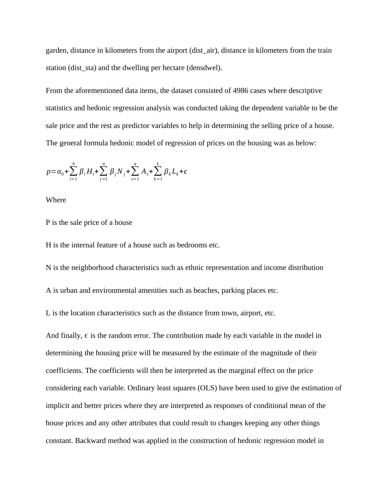
garden, distance in kilometers from the airport (dist_air), distance in kilometers from the train
station (dist_sta) and the dwelling per hectare (densdwel).
From the aforementioned data items, the dataset consisted of 4986 cases where descriptive
statistics and hedonic regression analysis was conducted taking the dependent variable to be the
sale price and the rest as predictor variables to help in determining the selling price of a house.
The general formula hedonic model of regression of prices on the housing was as below:
p=α0 +∑
i=1
h
βi Hi+∑
j =1
n
β j N j +∑
s=1
a
As+∑
k=1
L
βk Lk +ϵ
Where
P is the sale price of a house
H is the internal feature of a house such as bedrooms etc.
N is the neighborhood characteristics such as ethnic representation and income distribution
A is urban and environmental amenities such as beaches, parking places etc.
L is the location characteristics such as the distance from town, airport, etc.
And finally, ϵ is the random error. The contribution made by each variable in the model in
determining the housing price will be measured by the estimate of the magnitude of their
coefficients. The coefficients will then be interpreted as the marginal effect on the price
considering each variable. Ordinary least squares (OLS) have been used to give the estimation of
implicit and better prices where they are interpreted as responses of conditional mean of the
house prices and any other attributes that could result to changes keeping any other things
constant. Backward method was applied in the construction of hedonic regression model in
checking for the variables that best fitted in predicting the price of a home. In the process,
predictors which was not affecting the selling price of a house would be removed and remain
with only ones that were affecting the dependent variable.
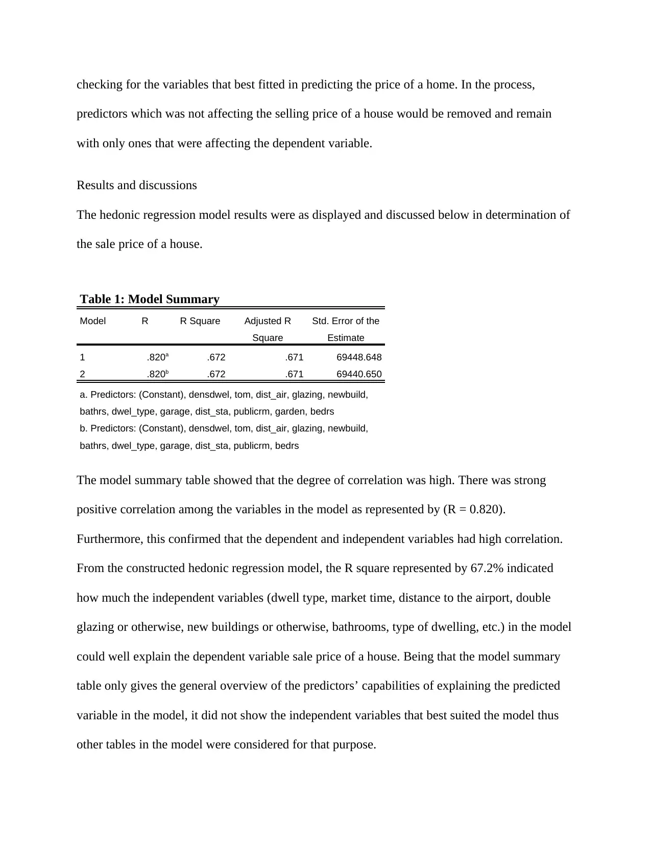
Results and discussions
The hedonic regression model results were as displayed and discussed below in determination of
the sale price of a house.
Table 1: Model Summary
Model R R Square Adjusted R
Square
Std. Error of the
Estimate
1 .820a .672 .671 69448.648
2 .820b .672 .671 69440.650
a. Predictors: (Constant), densdwel, tom, dist_air, glazing, newbuild,
bathrs, dwel_type, garage, dist_sta, publicrm, garden, bedrs
b. Predictors: (Constant), densdwel, tom, dist_air, glazing, newbuild,
bathrs, dwel_type, garage, dist_sta, publicrm, bedrs
The model summary table showed that the degree of correlation was high. There was strong
positive correlation among the variables in the model as represented by (R = 0.820).
Furthermore, this confirmed that the dependent and independent variables had high correlation.
From the constructed hedonic regression model, the R square represented by 67.2% indicated
how much the independent variables (dwell type, market time, distance to the airport, double
glazing or otherwise, new buildings or otherwise, bathrooms, type of dwelling, etc.) in the model
could well explain the dependent variable sale price of a house. Being that the model summary
table only gives the general overview of the predictors’ capabilities of explaining the predicted
variable in the model, it did not show the independent variables that best suited the model thus
other tables in the model were considered for that purpose.
predictors which was not affecting the selling price of a house would be removed and remain
with only ones that were affecting the dependent variable.
Results and discussions
The hedonic regression model results were as displayed and discussed below in determination of
the sale price of a house.
Table 1: Model Summary
Model R R Square Adjusted R
Square
Std. Error of the
Estimate
1 .820a .672 .671 69448.648
2 .820b .672 .671 69440.650
a. Predictors: (Constant), densdwel, tom, dist_air, glazing, newbuild,
bathrs, dwel_type, garage, dist_sta, publicrm, garden, bedrs
b. Predictors: (Constant), densdwel, tom, dist_air, glazing, newbuild,
bathrs, dwel_type, garage, dist_sta, publicrm, bedrs
The model summary table showed that the degree of correlation was high. There was strong
positive correlation among the variables in the model as represented by (R = 0.820).
Furthermore, this confirmed that the dependent and independent variables had high correlation.
From the constructed hedonic regression model, the R square represented by 67.2% indicated
how much the independent variables (dwell type, market time, distance to the airport, double
glazing or otherwise, new buildings or otherwise, bathrooms, type of dwelling, etc.) in the model
could well explain the dependent variable sale price of a house. Being that the model summary
table only gives the general overview of the predictors’ capabilities of explaining the predicted
variable in the model, it did not show the independent variables that best suited the model thus
other tables in the model were considered for that purpose.
⊘ This is a preview!⊘
Do you want full access?
Subscribe today to unlock all pages.
Trusted by 1+ million students worldwide
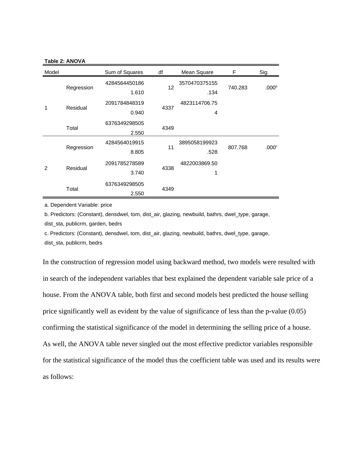
Table 2: ANOVA
Model Sum of Squares df Mean Square F Sig.
1
Regression 4284564450186
1.610 12 3570470375155
.134 740.283 .000b
Residual 2091784848319
0.940 4337 4823114706.75
4
Total 6376349298505
2.550 4349
2
Regression 4284564019915
8.805 11 3895058199923
.528 807.768 .000c
Residual 2091785278589
3.740 4338 4822003869.50
1
Total 6376349298505
2.550 4349
a. Dependent Variable: price
b. Predictors: (Constant), densdwel, tom, dist_air, glazing, newbuild, bathrs, dwel_type, garage,
dist_sta, publicrm, garden, bedrs
c. Predictors: (Constant), densdwel, tom, dist_air, glazing, newbuild, bathrs, dwel_type, garage,
dist_sta, publicrm, bedrs
In the construction of regression model using backward method, two models were resulted with
in search of the independent variables that best explained the dependent variable sale price of a
house. From the ANOVA table, both first and second models best predicted the house selling
price significantly well as evident by the value of significance of less than the p-value (0.05)
confirming the statistical significance of the model in determining the selling price of a house.
As well, the ANOVA table never singled out the most effective predictor variables responsible
for the statistical significance of the model thus the coefficient table was used and its results were
as follows:
Paraphrase This Document
Need a fresh take? Get an instant paraphrase of this document with our AI Paraphraser
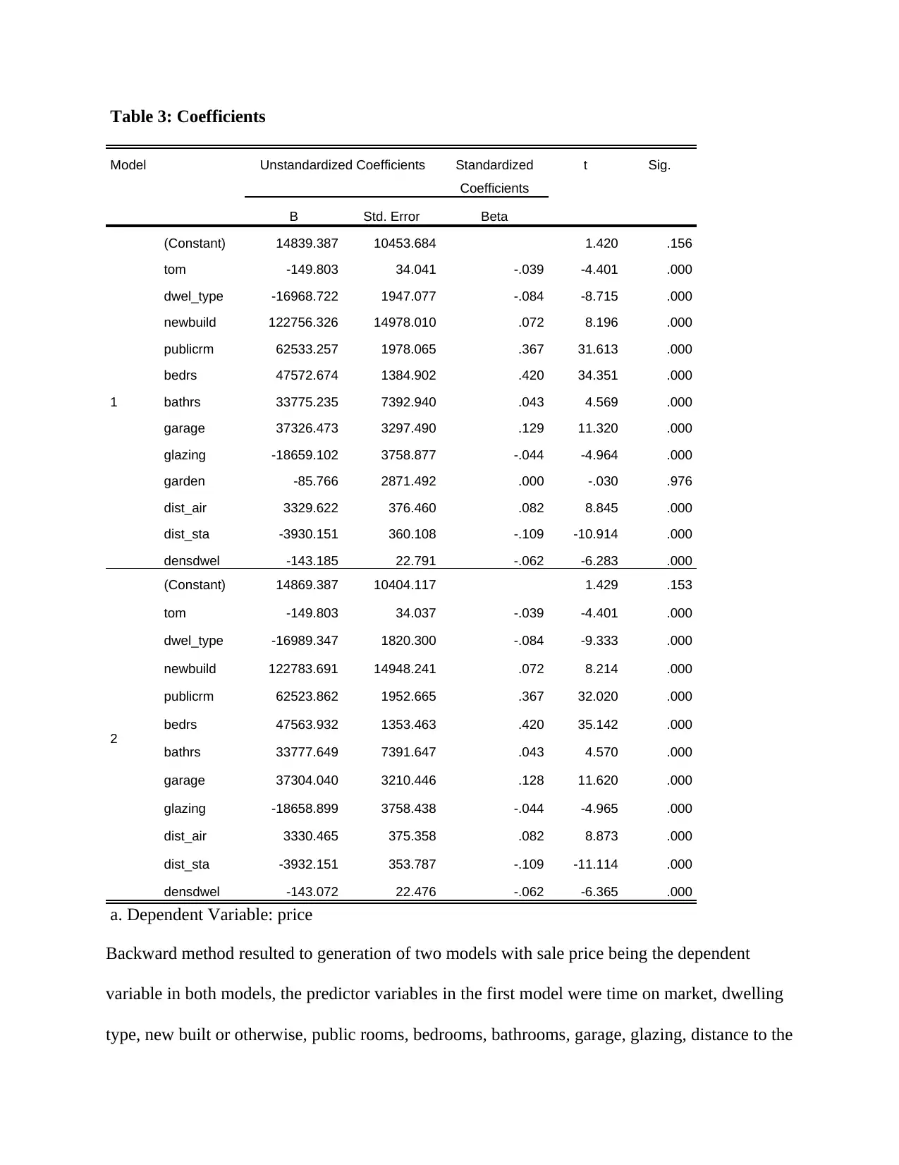
Table 3: Coefficients
Model Unstandardized Coefficients Standardized
Coefficients
t Sig.
B Std. Error Beta
1
(Constant) 14839.387 10453.684 1.420 .156
tom -149.803 34.041 -.039 -4.401 .000
dwel_type -16968.722 1947.077 -.084 -8.715 .000
newbuild 122756.326 14978.010 .072 8.196 .000
publicrm 62533.257 1978.065 .367 31.613 .000
bedrs 47572.674 1384.902 .420 34.351 .000
bathrs 33775.235 7392.940 .043 4.569 .000
garage 37326.473 3297.490 .129 11.320 .000
glazing -18659.102 3758.877 -.044 -4.964 .000
garden -85.766 2871.492 .000 -.030 .976
dist_air 3329.622 376.460 .082 8.845 .000
dist_sta -3930.151 360.108 -.109 -10.914 .000
densdwel -143.185 22.791 -.062 -6.283 .000
2
(Constant) 14869.387 10404.117 1.429 .153
tom -149.803 34.037 -.039 -4.401 .000
dwel_type -16989.347 1820.300 -.084 -9.333 .000
newbuild 122783.691 14948.241 .072 8.214 .000
publicrm 62523.862 1952.665 .367 32.020 .000
bedrs 47563.932 1353.463 .420 35.142 .000
bathrs 33777.649 7391.647 .043 4.570 .000
garage 37304.040 3210.446 .128 11.620 .000
glazing -18658.899 3758.438 -.044 -4.965 .000
dist_air 3330.465 375.358 .082 8.873 .000
dist_sta -3932.151 353.787 -.109 -11.114 .000
densdwel -143.072 22.476 -.062 -6.365 .000
a. Dependent Variable: price
Backward method resulted to generation of two models with sale price being the dependent
variable in both models, the predictor variables in the first model were time on market, dwelling
type, new built or otherwise, public rooms, bedrooms, bathrooms, garage, glazing, distance to the
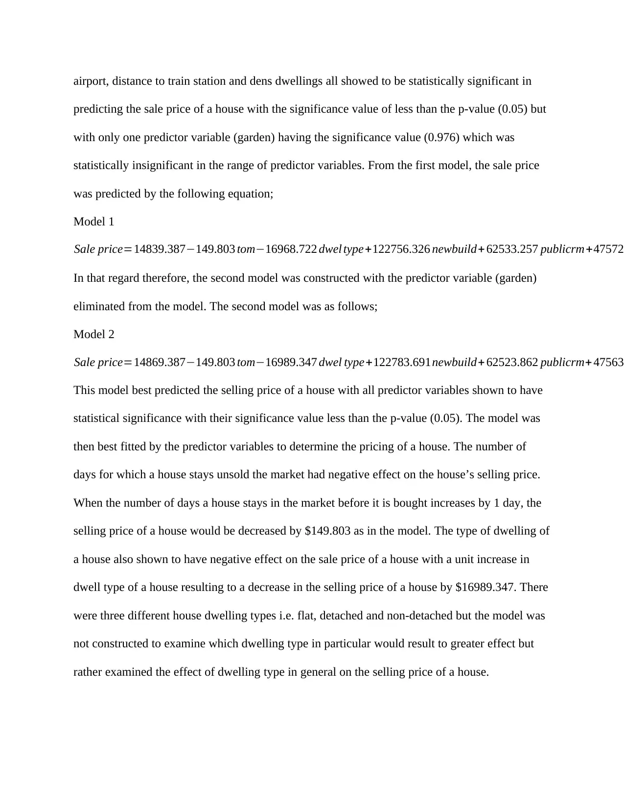
airport, distance to train station and dens dwellings all showed to be statistically significant in
predicting the sale price of a house with the significance value of less than the p-value (0.05) but
with only one predictor variable (garden) having the significance value (0.976) which was
statistically insignificant in the range of predictor variables. From the first model, the sale price
was predicted by the following equation;
Model 1
Sale price=14839.387−149.803 tom−16968.722 dwel type+122756.326 newbuild+ 62533.257 publicrm+47572.
In that regard therefore, the second model was constructed with the predictor variable (garden)
eliminated from the model. The second model was as follows;
Model 2
Sale price=14869.387−149.803 tom−16989.347 dwel type+122783.691newbuild+ 62523.862 publicrm+ 47563.
This model best predicted the selling price of a house with all predictor variables shown to have
statistical significance with their significance value less than the p-value (0.05). The model was
then best fitted by the predictor variables to determine the pricing of a house. The number of
days for which a house stays unsold the market had negative effect on the house’s selling price.
When the number of days a house stays in the market before it is bought increases by 1 day, the
selling price of a house would be decreased by $149.803 as in the model. The type of dwelling of
a house also shown to have negative effect on the sale price of a house with a unit increase in
dwell type of a house resulting to a decrease in the selling price of a house by $16989.347. There
were three different house dwelling types i.e. flat, detached and non-detached but the model was
not constructed to examine which dwelling type in particular would result to greater effect but
rather examined the effect of dwelling type in general on the selling price of a house.
⊘ This is a preview!⊘
Do you want full access?
Subscribe today to unlock all pages.
Trusted by 1+ million students worldwide
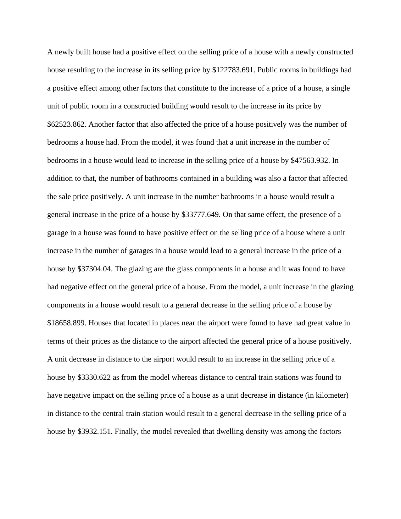
A newly built house had a positive effect on the selling price of a house with a newly constructed
house resulting to the increase in its selling price by $122783.691. Public rooms in buildings had
a positive effect among other factors that constitute to the increase of a price of a house, a single
unit of public room in a constructed building would result to the increase in its price by
$62523.862. Another factor that also affected the price of a house positively was the number of
bedrooms a house had. From the model, it was found that a unit increase in the number of
bedrooms in a house would lead to increase in the selling price of a house by $47563.932. In
addition to that, the number of bathrooms contained in a building was also a factor that affected
the sale price positively. A unit increase in the number bathrooms in a house would result a
general increase in the price of a house by $33777.649. On that same effect, the presence of a
garage in a house was found to have positive effect on the selling price of a house where a unit
increase in the number of garages in a house would lead to a general increase in the price of a
house by $37304.04. The glazing are the glass components in a house and it was found to have
had negative effect on the general price of a house. From the model, a unit increase in the glazing
components in a house would result to a general decrease in the selling price of a house by
$18658.899. Houses that located in places near the airport were found to have had great value in
terms of their prices as the distance to the airport affected the general price of a house positively.
A unit decrease in distance to the airport would result to an increase in the selling price of a
house by $3330.622 as from the model whereas distance to central train stations was found to
have negative impact on the selling price of a house as a unit decrease in distance (in kilometer)
in distance to the central train station would result to a general decrease in the selling price of a
house by $3932.151. Finally, the model revealed that dwelling density was among the factors
Paraphrase This Document
Need a fresh take? Get an instant paraphrase of this document with our AI Paraphraser
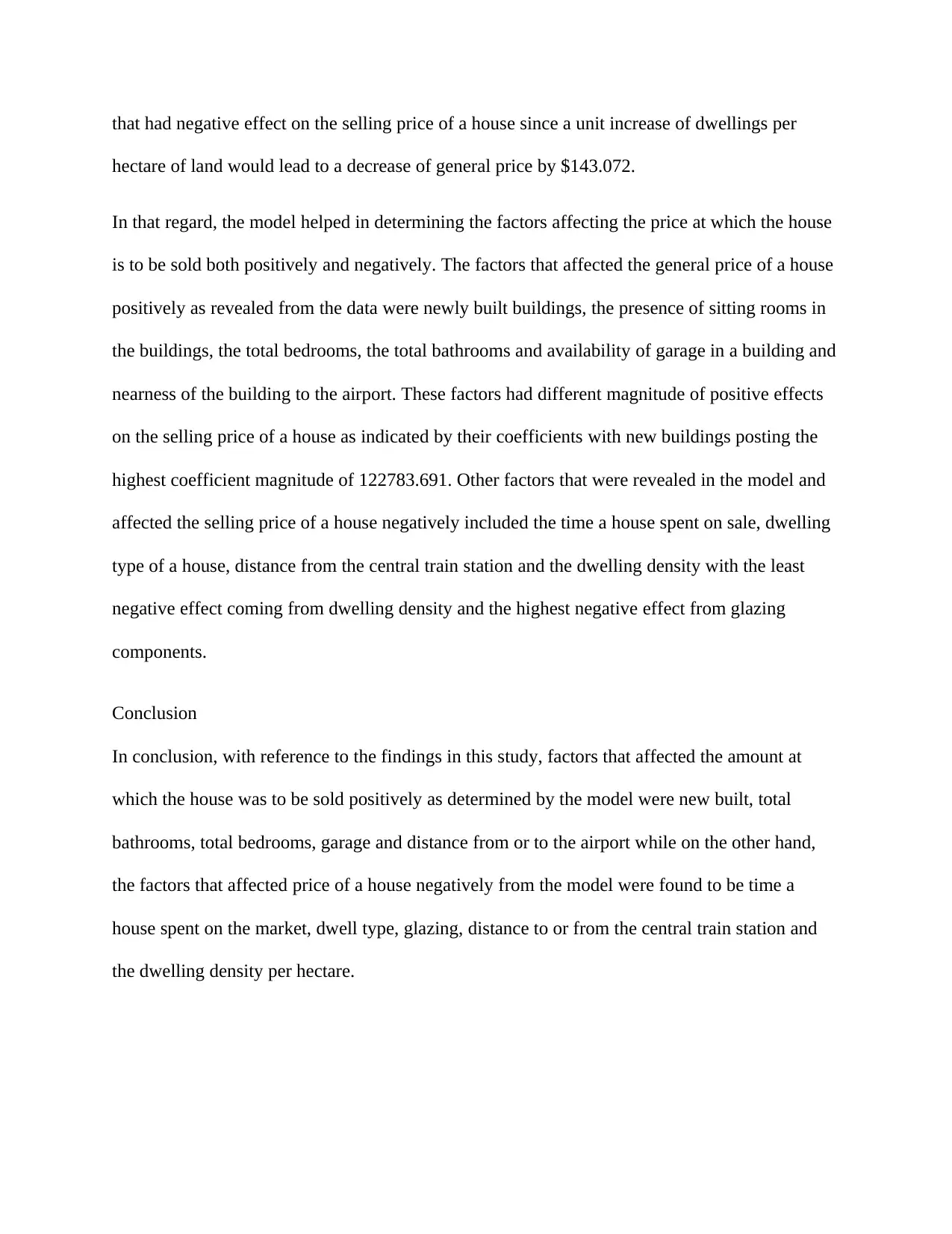
that had negative effect on the selling price of a house since a unit increase of dwellings per
hectare of land would lead to a decrease of general price by $143.072.
In that regard, the model helped in determining the factors affecting the price at which the house
is to be sold both positively and negatively. The factors that affected the general price of a house
positively as revealed from the data were newly built buildings, the presence of sitting rooms in
the buildings, the total bedrooms, the total bathrooms and availability of garage in a building and
nearness of the building to the airport. These factors had different magnitude of positive effects
on the selling price of a house as indicated by their coefficients with new buildings posting the
highest coefficient magnitude of 122783.691. Other factors that were revealed in the model and
affected the selling price of a house negatively included the time a house spent on sale, dwelling
type of a house, distance from the central train station and the dwelling density with the least
negative effect coming from dwelling density and the highest negative effect from glazing
components.
Conclusion
In conclusion, with reference to the findings in this study, factors that affected the amount at
which the house was to be sold positively as determined by the model were new built, total
bathrooms, total bedrooms, garage and distance from or to the airport while on the other hand,
the factors that affected price of a house negatively from the model were found to be time a
house spent on the market, dwell type, glazing, distance to or from the central train station and
the dwelling density per hectare.
References
Abrate, G. and Viglia, G., 2016. Strategic and tactical price decisions in hotel revenue
management. Tourism Management, 55, pp.123-132.
Andonov, A., Eichholtz, P. and Kok, N., 2015. Intermediated investment management in private
markets: Evidence from pension fund investments in real estate. Journal of Financial
Markets, 22, pp.73-103.
Barde, J.P. and Pearce, D.W., 2013. Valuing the environment: six case studies. Routledge.
Coulson, N.E. and Zabel, J.E., 2013. What can we learn from hedonic models when housing
markets are dominated by foreclosures?. Annu. Rev. Resour. Econ., 5(1), pp.261-279.
Del Giudice, V., Manganelli, B. and De Paola, P., 2017. Hedonic analysis of housing sales prices
with semiparametric methods. International Journal of Agricultural and Environmental
Information Systems (IJAEIS), 8(2), pp.65-77.
Del Giudice, V., Manganelli, B. and De Paola, P., 2015, June. Spline smoothing for estimating
hedonic housing price models. In International Conference on Computational Science and Its
Applications (pp. 210-219). Springer, Cham.
Estrella Orrego, M.J., Defrancesco, E. and Gennari, A., 2012. The wine hedonic price models in
the" Old and New World": state of the art. Revista de la Facultad de Ciencias Agrarias, 44(1).
Helbich, M., Brunauer, W., Vaz, E. and Nijkamp, P., 2014. Spatial heterogeneity in hedonic
house price models: the case of Austria. Urban Studies, 51(2), pp.390-411.
Hyland, M., Lyons, R.C. and Lyons, S., 2013. The value of domestic building energy efficiency
—evidence from Ireland. Energy Economics, 40, pp.943-952.
⊘ This is a preview!⊘
Do you want full access?
Subscribe today to unlock all pages.
Trusted by 1+ million students worldwide
1 out of 13
Related Documents


Your All-in-One AI-Powered Toolkit for Academic Success.
+13062052269
info@desklib.com
Available 24*7 on WhatsApp / Email
![[object Object]](/_next/static/media/star-bottom.7253800d.svg)
Unlock your academic potential
Copyright © 2020–2026 A2Z Services. All Rights Reserved. Developed and managed by ZUCOL.