Mechanical Engineering: Hewitt and Robert Flow Regime Analysis Report

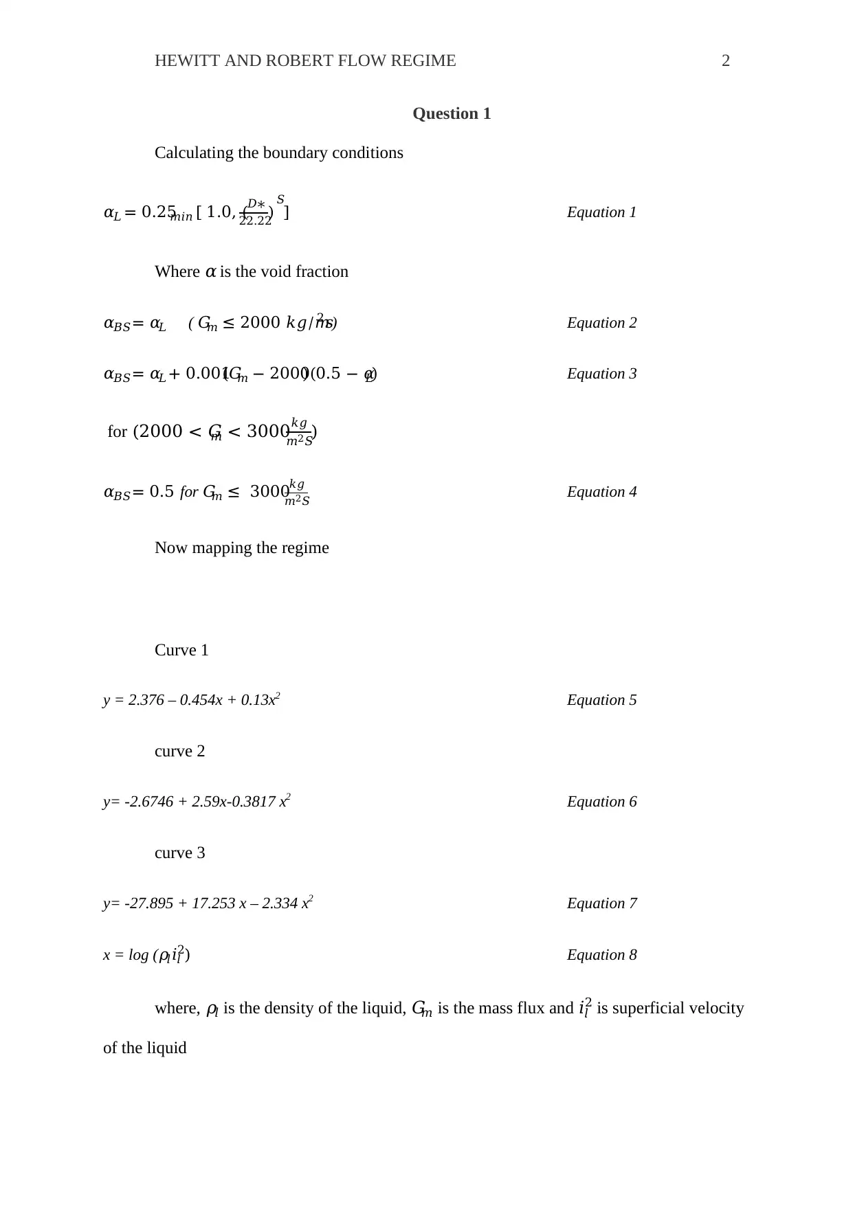
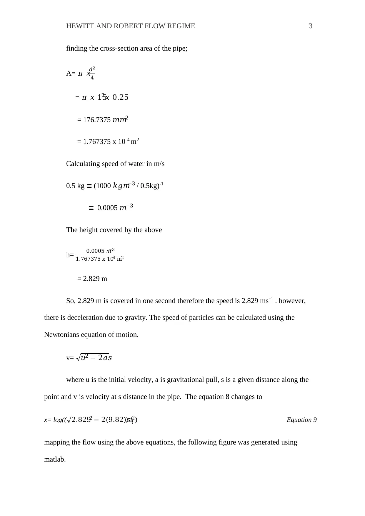
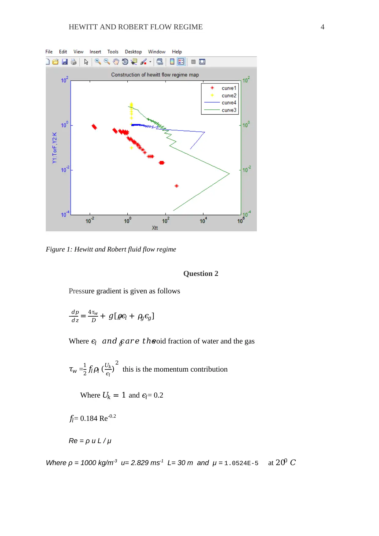
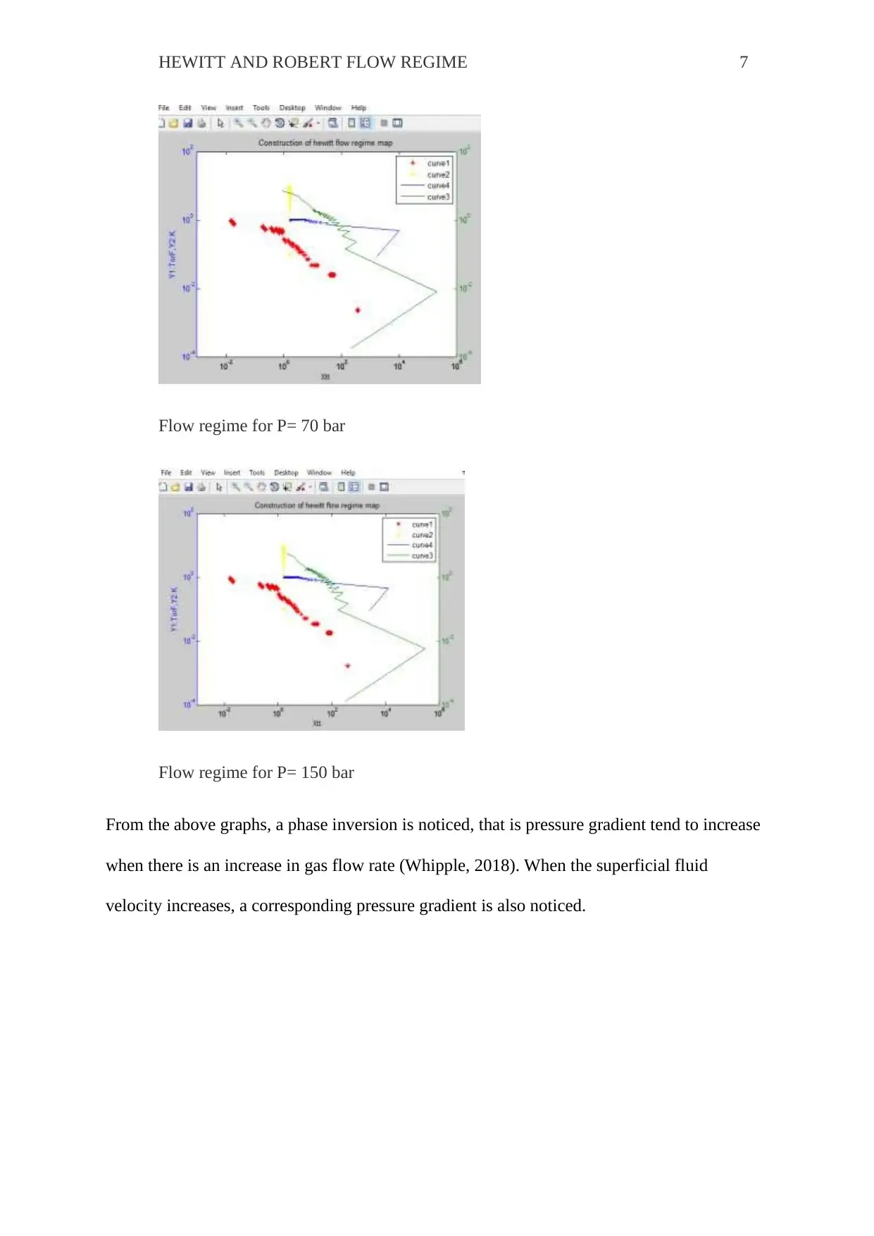
This report analyzes the Hewitt and Robert flow regime, focusing on fluid flow characteristics in vertical tubes. It begins by calculating boundary conditions and mapping the flow regime using provided equations, including the calculation of water speed and the application of Newtonian equations of motion. The report then addresses pressure gradient calculations, detailing the momentum contribution and determining pressure drop over a specified distance. Furthermore, it examines the critical heat flux, comparing densities and calculating mass flux. Finally, the report considers the impact of pressure changes on the flow regime, observing phase inversion at different pressure levels, and concludes with references to relevant literature. This report provides a comprehensive analysis of fluid flow dynamics, supported by calculations and graphical representations, and offers insights into the behavior of flow regimes under varying conditions.

Running Head: HEWITT AND ROBERT FLOW REGIME
HEWITT AND ROBERT FLOW REGIME
Name
Institute of Affiliation
Date

HEWITT AND ROBERT FLOW REGIME 2
Question 1
Calculating the boundary conditions
𝛼𝐿 = 0.25𝑚𝑖𝑛 [ 1.0, (𝐷∗
22.22
)𝑆
] Equation 1
Where 𝛼 is the void fraction
𝛼𝐵𝑆= 𝛼𝐿 ( 𝐺𝑚 ≤ 2000 𝑘𝑔/𝑚2𝑠) Equation 2
𝛼𝐵𝑆= 𝛼𝐿 + 0.001(𝐺𝑚 − 2000)(0.5 − 𝛼𝐿) Equation 3
for (2000 < 𝐺𝑚 < 3000𝑘𝑔
𝑚2𝑆)
𝛼𝐵𝑆= 0.5 for 𝐺𝑚 ≤ 3000𝑘𝑔
𝑚2𝑆 Equation 4
Now mapping the regime
Curve 1
y = 2.376 – 0.454x + 0.13x2 Equation 5
curve 2
y= -2.6746 + 2.59x-0.3817 x2 Equation 6
curve 3
y= -27.895 + 17.253 x – 2.334 x2 Equation 7
x = log (𝜌𝑙𝑖𝑙
2) Equation 8
where, 𝜌𝑙 is the density of the liquid, 𝐺𝑚 is the mass flux and 𝑖𝑙
2 is superficial velocity
of the liquid

HEWITT AND ROBERT FLOW REGIME 3
finding the cross-section area of the pipe;
A= 𝜋 𝑥
𝑑2
4
= 𝜋 𝑥 152𝑥 0.25
= 176.7375 𝑚𝑚2
= 1.767375 x 10-4 m2
Calculating speed of water in m/s
0.5 kg ≡ (1000 𝑘𝑔𝑚−3 / 0.5kg)-1
≡ 0.0005 𝑚−3
The height covered by the above
h= 0.0005 𝑚−3
1.767375 x 10−4 m2
= 2.829 m
So, 2.829 m is covered in one second therefore the speed is 2.829 ms-1 . however,
there is deceleration due to gravity. The speed of particles can be calculated using the
Newtonians equation of motion.
v= √𝑢2 − 2𝑎𝑠
where u is the initial velocity, a is gravitational pull, s is a given distance along the
point and v is velocity at s distance in the pipe. The equation 8 changes to
x= log((√2.8292 − 2(9.82)𝑠) 𝑖𝑙
2) Equation 9
mapping the flow using the above equations, the following figure was generated using
matlab.

HEWITT AND ROBERT FLOW REGIME 4
Figure 1: Hewitt and Robert fluid flow regime
Question 2
Pressure gradient is given as follows
-𝑑𝑝
𝑑𝑧 = 4𝜏𝑤
𝐷 + 𝑔[𝜌𝑙𝜖𝑙 + 𝜌𝑔𝜖𝑔]
Where 𝜖𝑙 𝑎𝑛𝑑 𝜖𝑔 𝑎𝑟𝑒 𝑡ℎ𝑒void fraction of water and the gas
𝜏𝑤 =1
2 𝑓𝑙𝜌𝑙 (𝑈𝑘
𝜖𝑙
)2
this is the momentum contribution
Where 𝑈𝑘 = 1 and 𝜖𝑙= 0.2
𝑓𝑙= 0.184 Re-0.2
Re = ρ u L / μ
Where ρ = 1000 kg/m-3 u= 2.829 ms-1 L= 30 m and μ = 1.0524E-5 at 200 𝐶

HEWITT AND ROBERT FLOW REGIME 5
Re = 1000 𝑥 2.829 𝑥 30
1.0524x 10−5
= 8.0675 x 10^9
Fl = 0.184 𝑥(8.0675 𝑥 109)−2
= 0.0019
𝜏𝑤 becomes as follows;
𝜏𝑤 =1
2 𝑓𝑙𝜌𝑙 (𝑈𝑘
𝜖𝑙
)2
= 1
2 𝑥 0.0019 𝑥 1000 (
1
0.2
)2
= 24.0093
Therefore, pressure drop becomes
− 𝑑𝑝
𝑑𝑧 = 4𝜏𝑤
𝐷 + 𝑔[𝜌𝑙𝜖𝑙 + 𝜌𝑔𝜖𝑔]
= (4∗24.0093)
0.015 + 9.82 ∗ (1000 ∗ 0.2 + 1.28 ∗ 0.046 )
= 8.3671 x 1003 Pa/m
Therefore, pressure drop in 30 m will
𝑑𝑝30 = 8.3671 x 1003 Pa
m x30 m
= 2.5101x 105 pa
≡ 2.5101 𝑏𝑎𝑟𝑠

HEWITT AND ROBERT FLOW REGIME 6
Question 3
ESDU 86032a pdf has not been provided
The ratio of density of liquid and gas
The density of are 𝜌𝑔= 1.23 kg/m^3
The density of the liquid 𝜌𝑙= 1000 kg/m^3
𝜌𝑙
𝜌𝑔
= 813.34
The mass flux
𝑚̇ = 4𝑀̇
𝜋𝐷2𝑁𝑇
= 4 𝑥 0.5
𝜋∗0.0152∗1
= 2829.1 𝑘𝑔𝑠−1𝑚−2
𝑥𝑔 𝑜𝑢𝑡 ,= 0.8 𝐵𝑜𝑐𝑟 ∗× 106 = 2834
𝑞 ∗𝑐𝑟= 𝑚𝑎𝑠𝑠 𝑓𝑙𝑢𝑥 ∗ 𝑥𝑜𝑢𝑡,𝑔∗ Δ ℎ
= 2829.1 x 2834 x 10−6 x 1078 x 103
= 8.6457x 103
Hence the critical heat flux is not exceeded.
Question 4
When pressure has been drop to 70 bars, the curve the flow regime appears as
follows;

HEWITT AND ROBERT FLOW REGIME 7
Flow regime for P= 70 bar
Flow regime for P= 150 bar
From the above graphs, a phase inversion is noticed, that is pressure gradient tend to increase
when there is an increase in gas flow rate (Whipple, 2018). When the superficial fluid
velocity increases, a corresponding pressure gradient is also noticed.

HEWITT AND ROBERT FLOW REGIME 8
References
Whipple, A. A. (2018). Managing flow regimes and landscapes together: Hydrospatial
analysis for evaluating spatiotemporal floodplain inundation patterns with
restoration and climate change implications.
Johnson, A. T., Micellie, T. M., Masaitis, C., & Edgewood Arsenal (Md.). (2013). Flow
Regimes in Protective Masks. Ft. Belvoir: Defense Technical Information Center.