HI6007 Statistics & Research Methods: Data Analysis and Interpretation

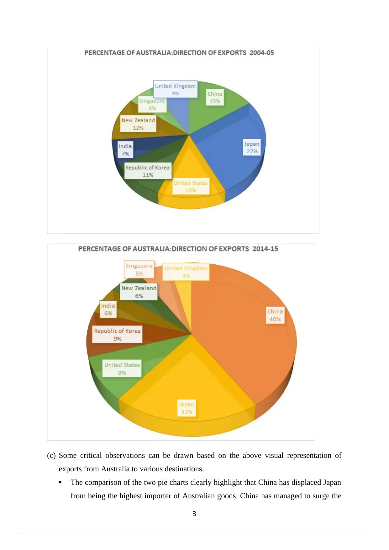
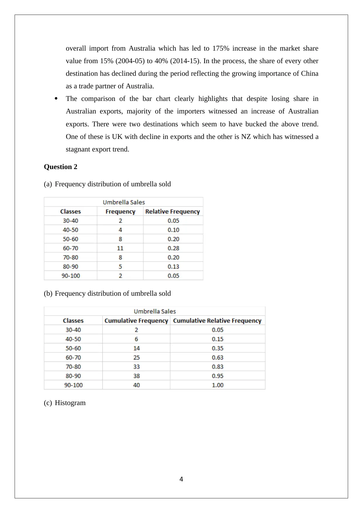
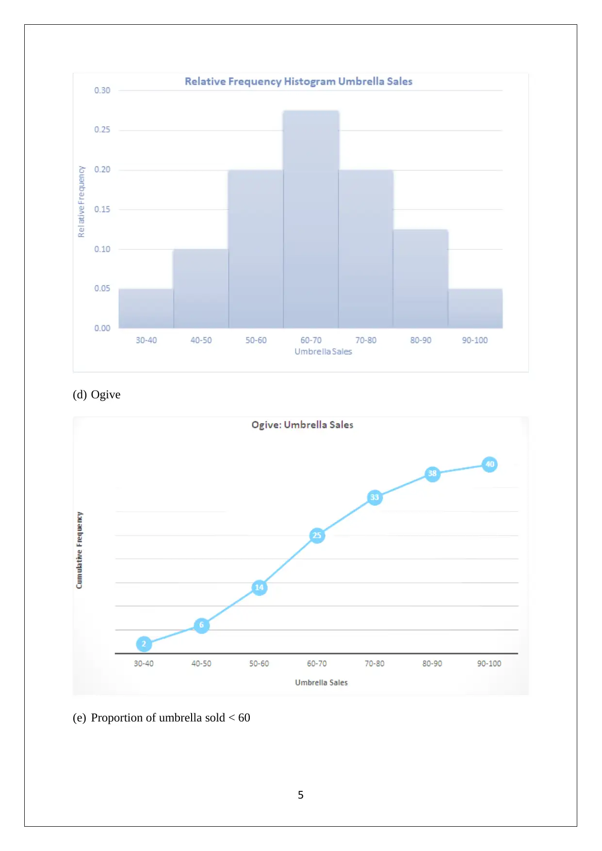
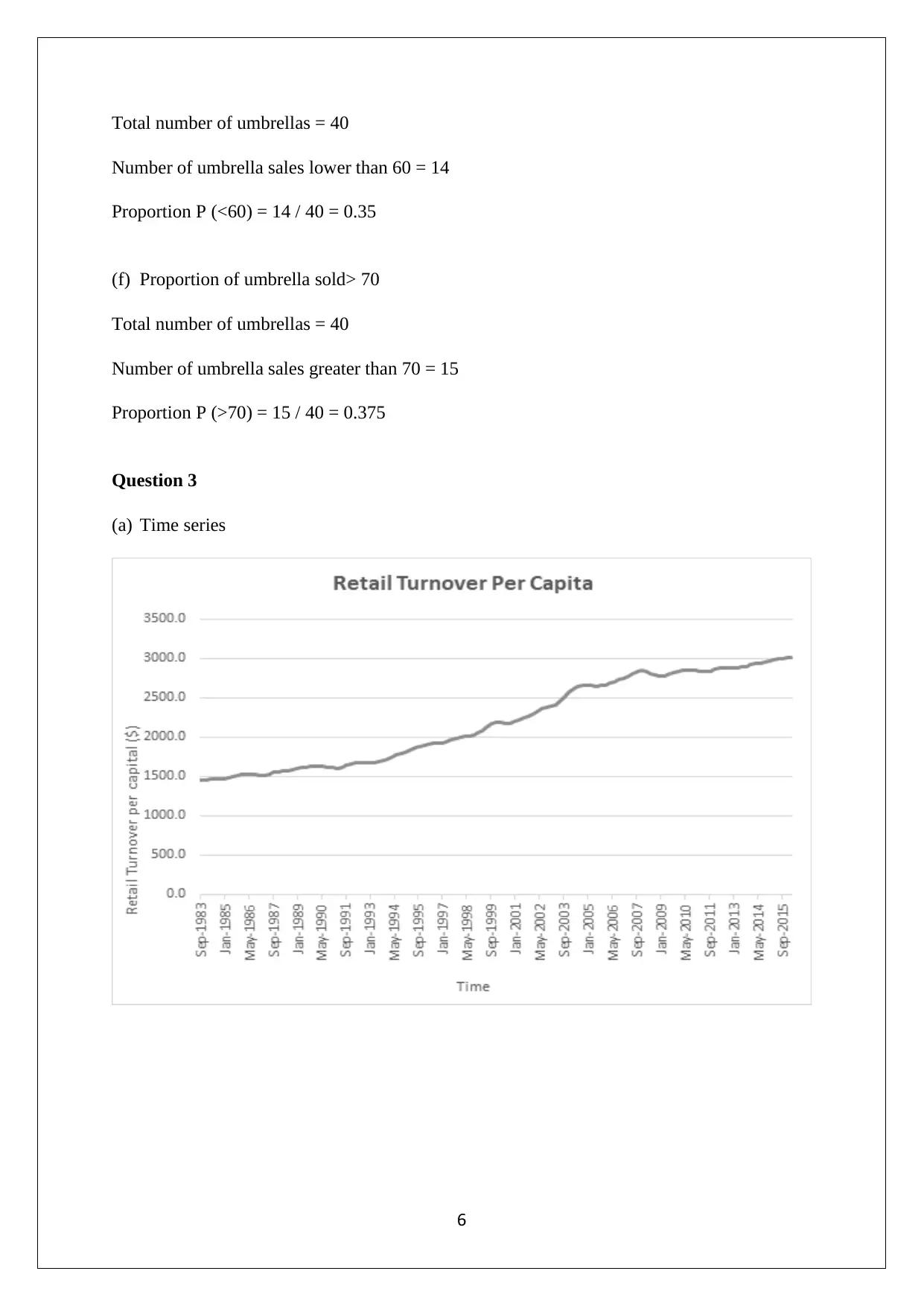
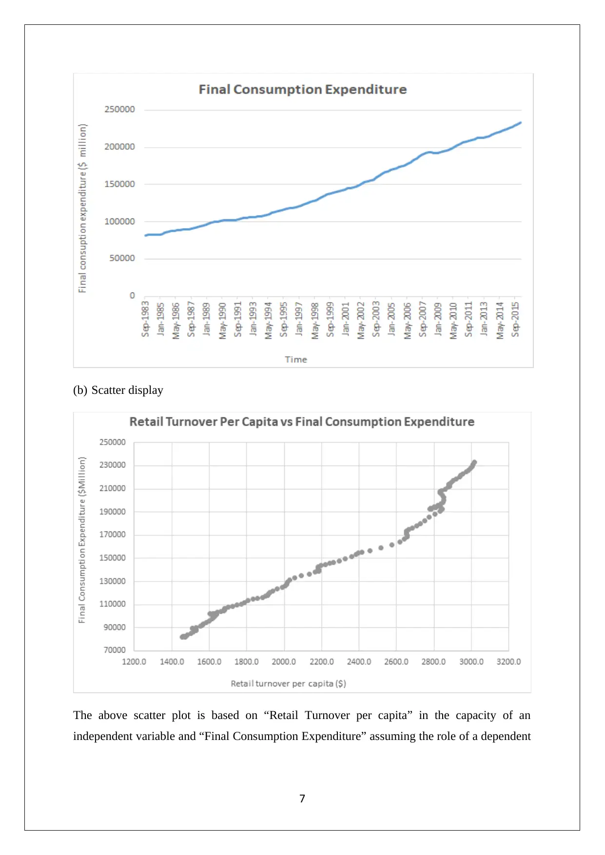
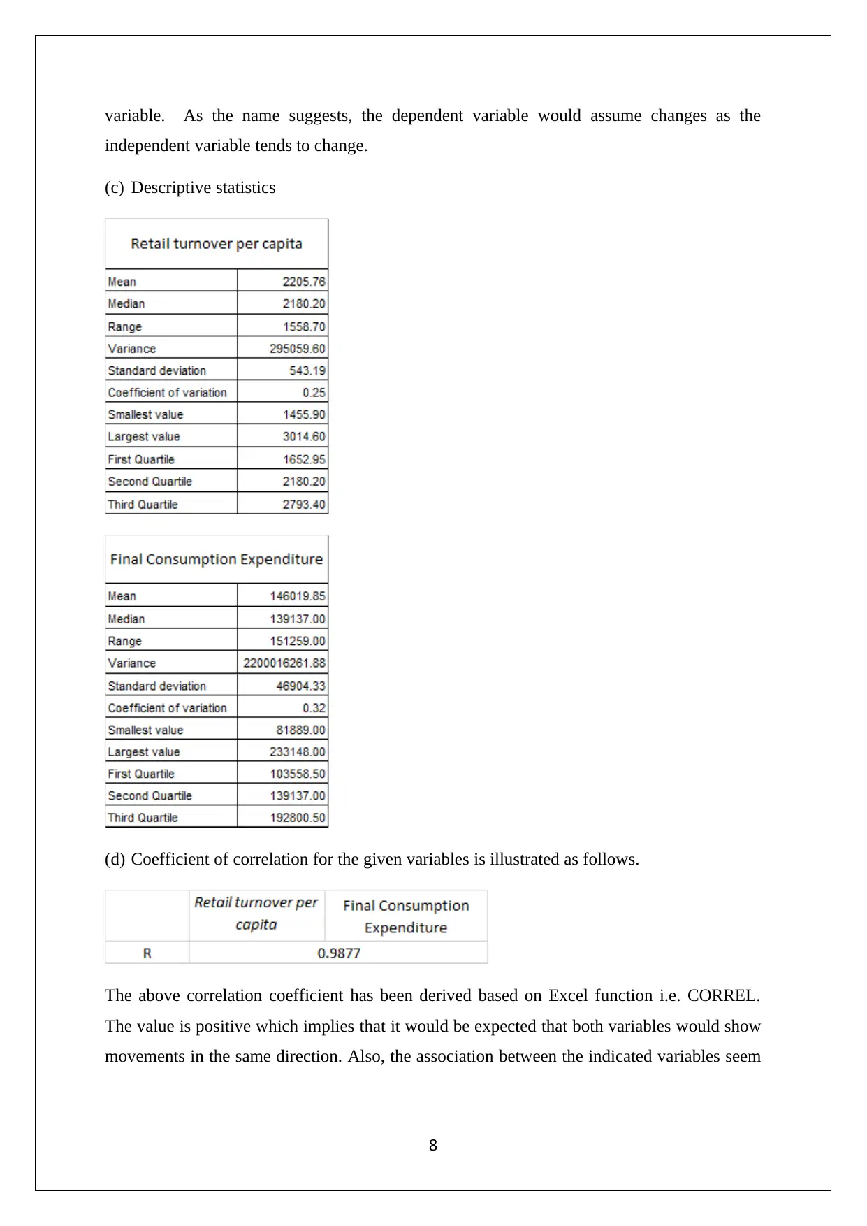
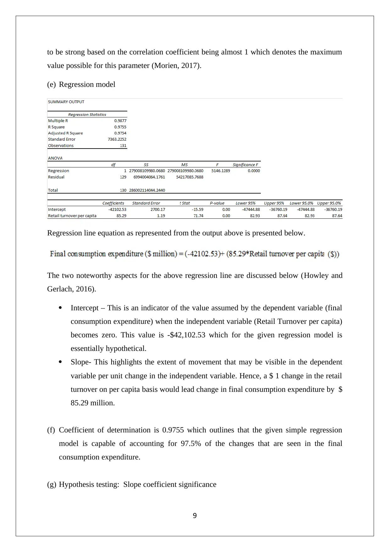
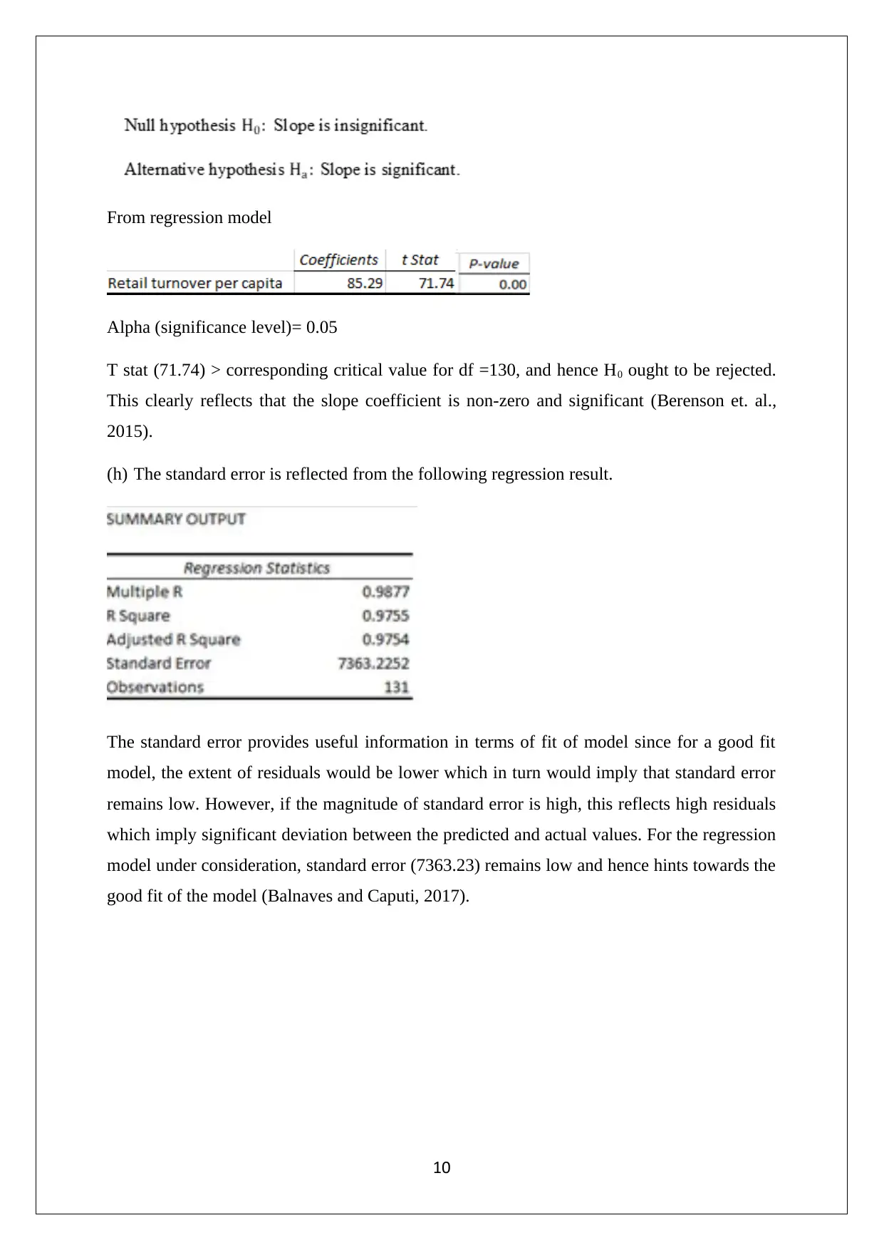
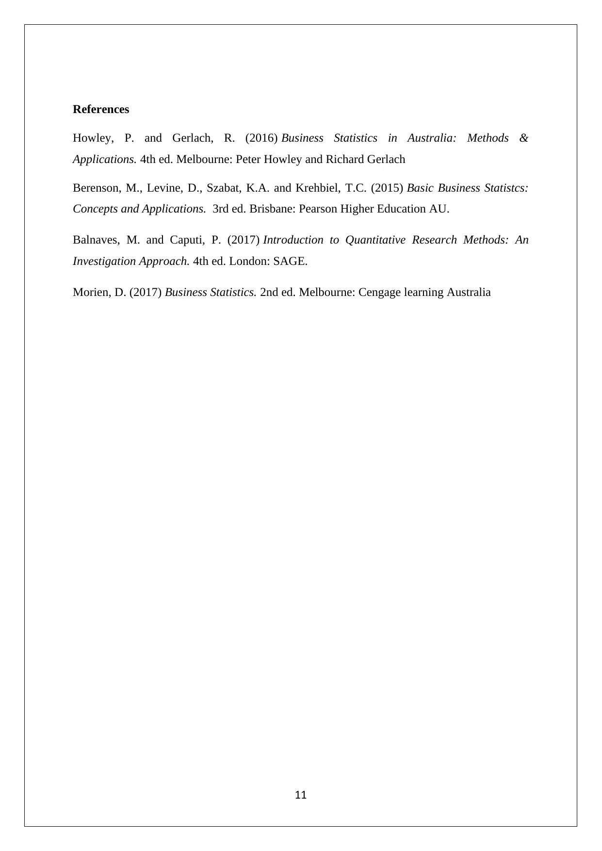
This assignment focuses on statistical analysis and interpretation of data, covering topics such as data visualization, frequency distribution, correlation, and regression analysis. It begins with an analysis of Australia's export data to various countries, using bar charts and pie charts to highlight trends and shifts in trade partnerships, particularly the rise of China as a major importer. The assignment then delves into frequency distributions and histograms related to umbrella sales, followed by a time series and scatter plot analysis of retail turnover per capita and final consumption expenditure. Descriptive statistics, correlation coefficients, regression models, and hypothesis testing are applied to the economic data, with interpretations of the results. The regression model's intercept, slope, coefficient of determination, and standard error are discussed in detail, providing a comprehensive understanding of the relationship between the variables. The assignment concludes with hypothesis testing to determine the significance of the slope coefficient.

STATISTICS
STUDENT ID:
[Pick the date]

Question 1
(a) The data for exports from Australia to various key destinations (importing countries) has
been summarised in the form of the following bar chart where one bar highlights the
exports from Australia to selected nations in 2004-05 while other bar highlights
corresponding exports in 2014-15.
(b) The representation of the above data with regards to percent share of each importing
country has been carried using pie chart for each of the two years of interest.
2

(c) Some critical observations can be drawn based on the above visual representation of
exports from Australia to various destinations.
 The comparison of the two pie charts clearly highlight that China has displaced Japan
from being the highest importer of Australian goods. China has managed to surge the
3

overall import from Australia which has led to 175% increase in the market share
value from 15% (2004-05) to 40% (2014-15). In the process, the share of every other
destination has declined during the period reflecting the growing importance of China
as a trade partner of Australia.
 The comparison of the bar chart clearly highlights that despite losing share in
Australian exports, majority of the importers witnessed an increase of Australian
exports. There were two destinations which seem to have bucked the above trend.
One of these is UK with decline in exports and the other is NZ which has witnessed a
stagnant export trend.
Question 2
(a) Frequency distribution of umbrella sold
(b) Frequency distribution of umbrella sold
(c) Histogram
4

(d) Ogive
(e) Proportion of umbrella sold < 60
5

Total number of umbrellas = 40
Number of umbrella sales lower than 60 = 14
Proportion P (<60) = 14 / 40 = 0.35
(f) Proportion of umbrella sold> 70
Total number of umbrellas = 40
Number of umbrella sales greater than 70 = 15
Proportion P (>70) = 15 / 40 = 0.375
Question 3
(a) Time series
6

(b) Scatter display
The above scatter plot is based on “Retail Turnover per capita” in the capacity of an
independent variable and “Final Consumption Expenditure” assuming the role of a dependent
7

variable. As the name suggests, the dependent variable would assume changes as the
independent variable tends to change.
(c) Descriptive statistics
(d) Coefficient of correlation for the given variables is illustrated as follows.
The above correlation coefficient has been derived based on Excel function i.e. CORREL.
The value is positive which implies that it would be expected that both variables would show
movements in the same direction. Also, the association between the indicated variables seem
8

to be strong based on the correlation coefficient being almost 1 which denotes the maximum
value possible for this parameter (Morien, 2017).
(e) Regression model
Regression line equation as represented from the output above is presented below.
The two noteworthy aspects for the above regression line are discussed below (Howley and
Gerlach, 2016).
 Intercept – This is an indicator of the value assumed by the dependent variable (final
consumption expenditure) when the independent variable (Retail Turnover per capita)
becomes zero. This value is -$42,102.53 which for the given regression model is
essentially hypothetical.
 Slope- This highlights the extent of movement that may be visible in the dependent
variable per unit change in the independent variable. Hence, a $ 1 change in the retail
turnover on per capita basis would lead change in final consumption expenditure by $
85.29 million.
(f) Coefficient of determination is 0.9755 which outlines that the given simple regression
model is capable of accounting for 97.5% of the changes that are seen in the final
consumption expenditure.
(g) Hypothesis testing: Slope coefficient significance
9

From regression model
Alpha (significance level)= 0.05
T stat (71.74) > corresponding critical value for df =130, and hence H0 ought to be rejected.
This clearly reflects that the slope coefficient is non-zero and significant (Berenson et. al.,
2015).
(h) The standard error is reflected from the following regression result.
The standard error provides useful information in terms of fit of model since for a good fit
model, the extent of residuals would be lower which in turn would imply that standard error
remains low. However, if the magnitude of standard error is high, this reflects high residuals
which imply significant deviation between the predicted and actual values. For the regression
model under consideration, standard error (7363.23) remains low and hence hints towards the
good fit of the model (Balnaves and Caputi, 2017).
10

References
Howley, P. and Gerlach, R. (2016) Business Statistics in Australia: Methods &
Applications. 4th ed. Melbourne: Peter Howley and Richard Gerlach
Berenson, M., Levine, D., Szabat, K.A. and Krehbiel, T.C. (2015) Basic Business Statistcs:
Concepts and Applications. 3rd ed. Brisbane: Pearson Higher Education AU.
Balnaves, M. and Caputi, P. (2017) Introduction to Quantitative Research Methods: An
Investigation Approach. 4th ed. London: SAGE.
Morien, D. (2017) Business Statistics. 2nd ed. Melbourne: Cengage learning Australia
11