HI6007 Statistics Assignment: Distribution, ANOVA, Regression
VerifiedAdded on 2024/06/03
|13
|2577
|92
Homework Assignment
AI Summary
This assignment solution covers various statistical concepts. It includes creating frequency, relative frequency, and percentage frequency distributions for furniture order data, constructing and interpreting histograms, and determining appropriate measures of location. The assignment also explores the relationship between demand and unit price using ANOVA, calculating the coefficient of determination and correlation. Furthermore, it involves developing and testing estimated regression equations to relate dependent and independent variables, interpreting slope coefficients, and conducting hypothesis tests. Desklib offers a wealth of similar solved assignments and study materials to aid students in their academic pursuits.
HI6007 Group Assignment
1
1
Paraphrase This Document
Need a fresh take? Get an instant paraphrase of this document with our AI Paraphraser
Contents
Question1..............................................................................................................................................2
Question 2.............................................................................................................................................5
Question 3.............................................................................................................................................8
Question 4.............................................................................................................................................9
References...........................................................................................................................................12
2
Question1
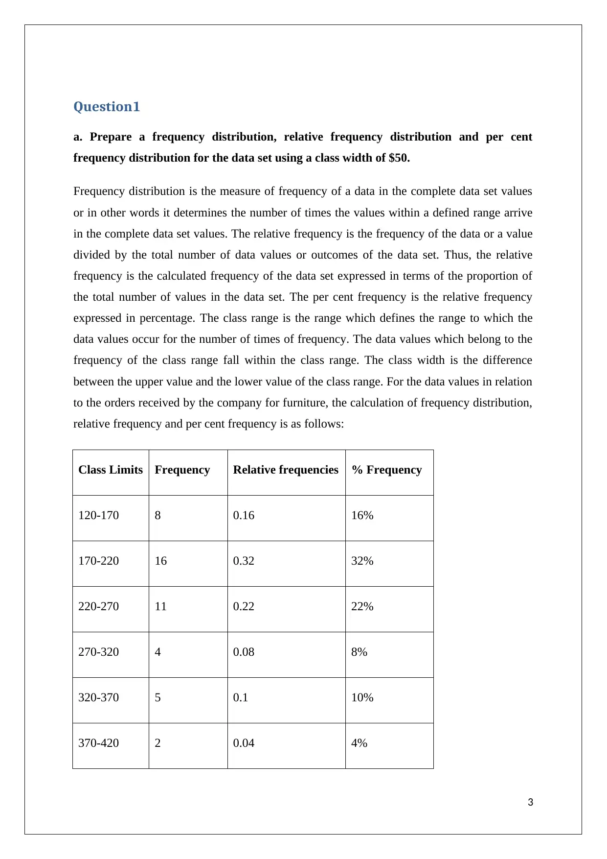
a. Prepare a frequency distribution, relative frequency distribution and per cent
frequency distribution for the data set using a class width of $50.
Frequency distribution is the measure of frequency of a data in the complete data set values
or in other words it determines the number of times the values within a defined range arrive
in the complete data set values. The relative frequency is the frequency of the data or a value
divided by the total number of data values or outcomes of the data set. Thus, the relative
frequency is the calculated frequency of the data set expressed in terms of the proportion of
the total number of values in the data set. The per cent frequency is the relative frequency
expressed in percentage. The class range is the range which defines the range to which the
data values occur for the number of times of frequency. The data values which belong to the
frequency of the class range fall within the class range. The class width is the difference
between the upper value and the lower value of the class range. For the data values in relation
to the orders received by the company for furniture, the calculation of frequency distribution,
relative frequency and per cent frequency is as follows:
Class Limits Frequency Relative frequencies % Frequency
120-170 8 0.16 16%
170-220 16 0.32 32%
220-270 11 0.22 22%
270-320 4 0.08 8%
320-370 5 0.1 10%
370-420 2 0.04 4%
3
⊘ This is a preview!⊘
Do you want full access?
Subscribe today to unlock all pages.
Trusted by 1+ million students worldwide
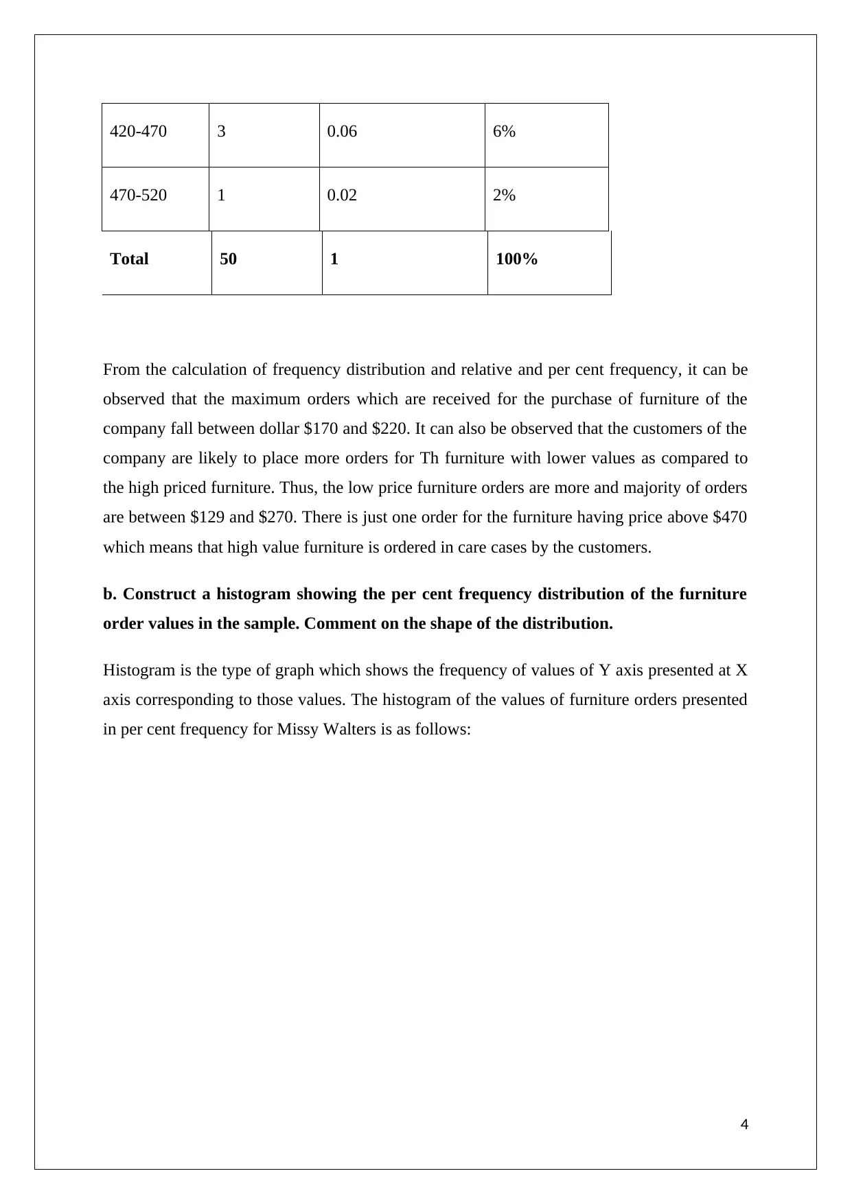
420-470 3 0.06 6%
470-520 1 0.02 2%
Total 50 1 100%
From the calculation of frequency distribution and relative and per cent frequency, it can be
observed that the maximum orders which are received for the purchase of furniture of the
company fall between dollar $170 and $220. It can also be observed that the customers of the
company are likely to place more orders for Th furniture with lower values as compared to
the high priced furniture. Thus, the low price furniture orders are more and majority of orders
are between $129 and $270. There is just one order for the furniture having price above $470
which means that high value furniture is ordered in care cases by the customers.
b. Construct a histogram showing the per cent frequency distribution of the furniture
order values in the sample. Comment on the shape of the distribution.
Histogram is the type of graph which shows the frequency of values of Y axis presented at X
axis corresponding to those values. The histogram of the values of furniture orders presented
in per cent frequency for Missy Walters is as follows:
4
Paraphrase This Document
Need a fresh take? Get an instant paraphrase of this document with our AI Paraphraser
1 2 3 4 5 6 7 8
0%
5%
10%
15%
20%
25%
30%
35%
Class Limits
Furniture orders
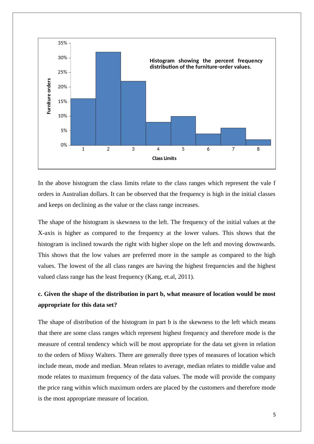
Histogram showing the percent frequency
distribution of the furniture-order values.
In the above histogram the class limits relate to the class ranges which represent the vale f
orders in Australian dollars. It can be observed that the frequency is high in the initial classes
and keeps on declining as the value or the class range increases.
The shape of the histogram is skewness to the left. The frequency of the initial values at the
X-axis is higher as compared to the frequency at the lower values. This shows that the
histogram is inclined towards the right with higher slope on the left and moving downwards.
This shows that the low values are preferred more in the sample as compared to the high
values. The lowest of the all class ranges are having the highest frequencies and the highest
valued class range has the least frequency (Kang, et.al, 2011).
c. Given the shape of the distribution in part b, what measure of location would be most
appropriate for this data set?
The shape of distribution of the histogram in part b is the skewness to the left which means
that there are some class ranges which represent highest frequency and therefore mode is the
measure of central tendency which will be most appropriate for the data set given in relation
to the orders of Missy Walters. There are generally three types of measures of location which
include mean, mode and median. Mean relates to average, median relates to middle value and
mode relates to maximum frequency of the data values. The mode will provide the company
the price rang within which maximum orders are placed by the customers and therefore mode
is the most appropriate measure of location.
5
0%
5%
10%
15%
20%
25%
30%
35%
Class Limits
Furniture orders
Histogram showing the percent frequency
distribution of the furniture-order values.
In the above histogram the class limits relate to the class ranges which represent the vale f
orders in Australian dollars. It can be observed that the frequency is high in the initial classes
and keeps on declining as the value or the class range increases.
The shape of the histogram is skewness to the left. The frequency of the initial values at the
X-axis is higher as compared to the frequency at the lower values. This shows that the
histogram is inclined towards the right with higher slope on the left and moving downwards.
This shows that the low values are preferred more in the sample as compared to the high
values. The lowest of the all class ranges are having the highest frequencies and the highest
valued class range has the least frequency (Kang, et.al, 2011).
c. Given the shape of the distribution in part b, what measure of location would be most
appropriate for this data set?
The shape of distribution of the histogram in part b is the skewness to the left which means
that there are some class ranges which represent highest frequency and therefore mode is the
measure of central tendency which will be most appropriate for the data set given in relation
to the orders of Missy Walters. There are generally three types of measures of location which
include mean, mode and median. Mean relates to average, median relates to middle value and
mode relates to maximum frequency of the data values. The mode will provide the company
the price rang within which maximum orders are placed by the customers and therefore mode
is the most appropriate measure of location.
5
Question 2
a. Determine whether or not demand and unit price are related.
ANOVA also known as the analysis of variance is the process which uses different types of
statistical models and approaches to identify and analyse the relationship which exists
between the mean values of different groups of data sets (Gu, 2013). It also analyses the
associated procedures of different groups such as variations, standard error etc. The demand
of a product is the quantity which is required by the customers in a particular market for a
specific product. The unit price is the price of each product at which the product can be sold
in the market to the customer. In economic terms there is an inverse relationship between
demand and unit price which means that when the price of a product increases the demand of
the product in the market falls and similarly on decrease in prices the demand accelerates.
However in statistical terms, the relationship cannot be established through mere observation
or analysis. The ANOVA tool can be used to measure the relationship. The ANOVA table
helps in the calculation of the F value which determines the degree of relationship between
the two variables or factors in relation to a product. The Following is the ANOVA table
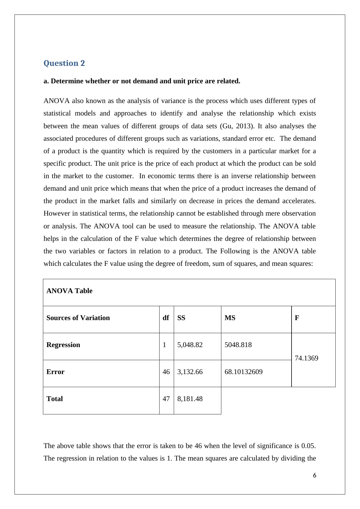
which calculates the F value using the degree of freedom, sum of squares, and mean squares:
ANOVA Table
Sources of Variation df SS MS F
Regression 1 5,048.82 5048.818
74.1369
Error 46 3,132.66 68.10132609
Total 47 8,181.48
The above table shows that the error is taken to be 46 when the level of significance is 0.05.
The regression in relation to the values is 1. The mean squares are calculated by dividing the
6
a. Determine whether or not demand and unit price are related.
ANOVA also known as the analysis of variance is the process which uses different types of
statistical models and approaches to identify and analyse the relationship which exists
between the mean values of different groups of data sets (Gu, 2013). It also analyses the
associated procedures of different groups such as variations, standard error etc. The demand
of a product is the quantity which is required by the customers in a particular market for a
specific product. The unit price is the price of each product at which the product can be sold
in the market to the customer. In economic terms there is an inverse relationship between
demand and unit price which means that when the price of a product increases the demand of
the product in the market falls and similarly on decrease in prices the demand accelerates.
However in statistical terms, the relationship cannot be established through mere observation
or analysis. The ANOVA tool can be used to measure the relationship. The ANOVA table
helps in the calculation of the F value which determines the degree of relationship between
the two variables or factors in relation to a product. The Following is the ANOVA table
which calculates the F value using the degree of freedom, sum of squares, and mean squares:
ANOVA Table
Sources of Variation df SS MS F
Regression 1 5,048.82 5048.818
74.1369
Error 46 3,132.66 68.10132609
Total 47 8,181.48
The above table shows that the error is taken to be 46 when the level of significance is 0.05.
The regression in relation to the values is 1. The mean squares are calculated by dividing the
6
⊘ This is a preview!⊘
Do you want full access?
Subscribe today to unlock all pages.
Trusted by 1+ million students worldwide
sum of squares by the degree of freedom. The F value calculated from the mean values of the
two variables is 74.1369. The F value is a high amount which shows that the degree of
relationship between the demand of the product and the unit price of the product is quite low.
Thus, it can be estimated that there is no relationship which exists between the demand of the
product and its unit price. Therefore if the market price of the product will be increased by
the seller, the demand of the product will not be affected. In economic terms these types of
products are defined as necessity goods.
b. Compute the coefficient of determination and fully interpret its meaning.
Coefficient of determination which is also known as the R-squared value is the measure
which defines the suitability of the data for the statistical model which is used for data
analysis (Hardle and Simar, 2012). The coefficient is when 1 means that the data perfectly
fits into the model and is indicated by a line in the graph and the coefficient when 0 indicates
that the data is highly inappropriate for the model and is represented by a curve in the graph.
The coefficient of determination helps identifying whether the specific statistical model can
be used for the data set or not. In this way it is used for the interpretation of suitability of
statistical model for a set of data values in order to select the appropriate statistical model for
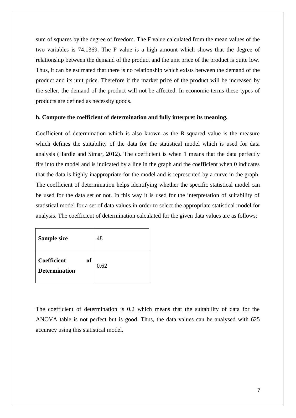
analysis. The coefficient of determination calculated for the given data values are as follows:
Sample size 48
Coefficient of
Determination 0.62
The coefficient of determination is 0.2 which means that the suitability of data for the
ANOVA table is not perfect but is good. Thus, the data values can be analysed with 625
accuracy using this statistical model.
7
two variables is 74.1369. The F value is a high amount which shows that the degree of
relationship between the demand of the product and the unit price of the product is quite low.
Thus, it can be estimated that there is no relationship which exists between the demand of the
product and its unit price. Therefore if the market price of the product will be increased by
the seller, the demand of the product will not be affected. In economic terms these types of
products are defined as necessity goods.
b. Compute the coefficient of determination and fully interpret its meaning.
Coefficient of determination which is also known as the R-squared value is the measure
which defines the suitability of the data for the statistical model which is used for data
analysis (Hardle and Simar, 2012). The coefficient is when 1 means that the data perfectly
fits into the model and is indicated by a line in the graph and the coefficient when 0 indicates
that the data is highly inappropriate for the model and is represented by a curve in the graph.
The coefficient of determination helps identifying whether the specific statistical model can
be used for the data set or not. In this way it is used for the interpretation of suitability of
statistical model for a set of data values in order to select the appropriate statistical model for
analysis. The coefficient of determination calculated for the given data values are as follows:
Sample size 48
Coefficient of
Determination 0.62
The coefficient of determination is 0.2 which means that the suitability of data for the
ANOVA table is not perfect but is good. Thus, the data values can be analysed with 625
accuracy using this statistical model.
7
Paraphrase This Document
Need a fresh take? Get an instant paraphrase of this document with our AI Paraphraser
c. Compute the coefficient of correlation and explain the relationship between demand
and unit price
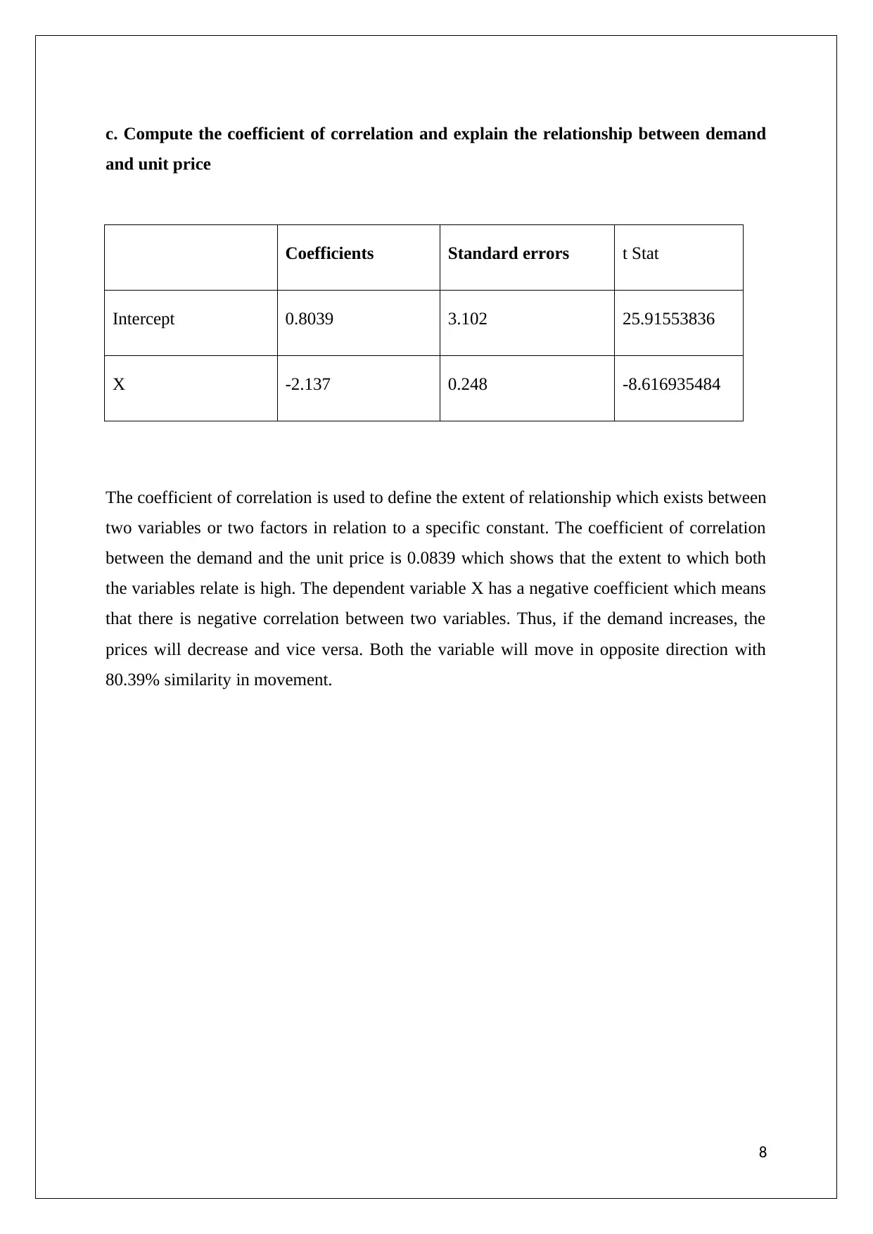
Coefficients Standard errors t Stat
Intercept 0.8039 3.102 25.91553836
X -2.137 0.248 -8.616935484
The coefficient of correlation is used to define the extent of relationship which exists between
two variables or two factors in relation to a specific constant. The coefficient of correlation
between the demand and the unit price is 0.0839 which shows that the extent to which both
the variables relate is high. The dependent variable X has a negative coefficient which means
that there is negative correlation between two variables. Thus, if the demand increases, the
prices will decrease and vice versa. Both the variable will move in opposite direction with
80.39% similarity in movement.
8
and unit price
Coefficients Standard errors t Stat
Intercept 0.8039 3.102 25.91553836
X -2.137 0.248 -8.616935484
The coefficient of correlation is used to define the extent of relationship which exists between
two variables or two factors in relation to a specific constant. The coefficient of correlation
between the demand and the unit price is 0.0839 which shows that the extent to which both
the variables relate is high. The dependent variable X has a negative coefficient which means
that there is negative correlation between two variables. Thus, if the demand increases, the
prices will decrease and vice versa. Both the variable will move in opposite direction with
80.39% similarity in movement.
8
Question 3
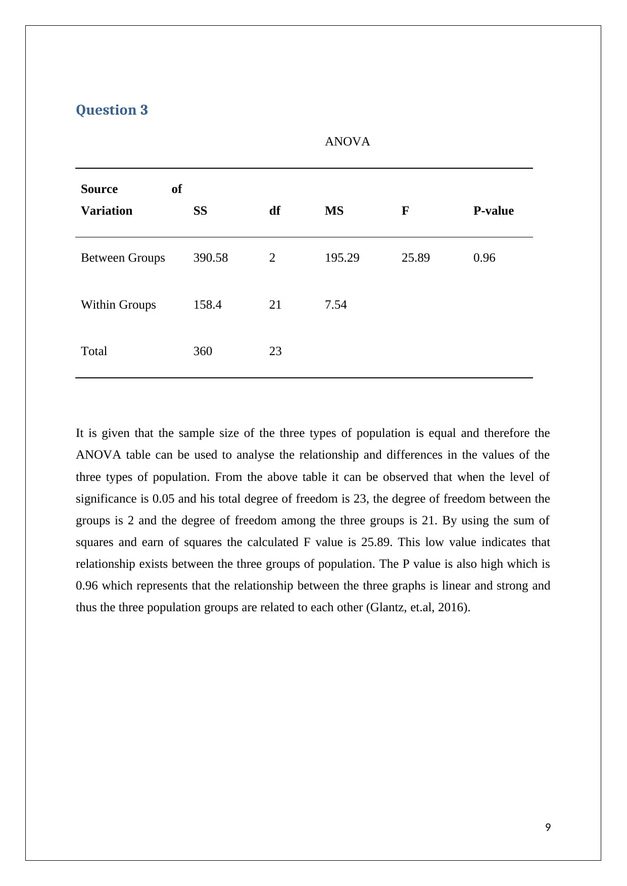
ANOVA
Source of
Variation SS df MS F P-value
Between Groups 390.58 2 195.29 25.89 0.96
Within Groups 158.4 21 7.54
Total 360 23
It is given that the sample size of the three types of population is equal and therefore the
ANOVA table can be used to analyse the relationship and differences in the values of the
three types of population. From the above table it can be observed that when the level of
significance is 0.05 and his total degree of freedom is 23, the degree of freedom between the
groups is 2 and the degree of freedom among the three groups is 21. By using the sum of
squares and earn of squares the calculated F value is 25.89. This low value indicates that
relationship exists between the three groups of population. The P value is also high which is
0.96 which represents that the relationship between the three graphs is linear and strong and
thus the three population groups are related to each other (Glantz, et.al, 2016).
9
⊘ This is a preview!⊘
Do you want full access?
Subscribe today to unlock all pages.
Trusted by 1+ million students worldwide
Question 4
a. Develop an estimated regression equation relating y to x1 and x2.
The number of mobile phones which are sold per day is represented by ( y). The price
related to y is represented by x1 and the number of advertising spots gathered for 7 days is
represented by X2. The estimated regression equation will be as follows:
Y = ax1 + x2
Here, a is the parameters which is constant and X1 and X2 will be variables.
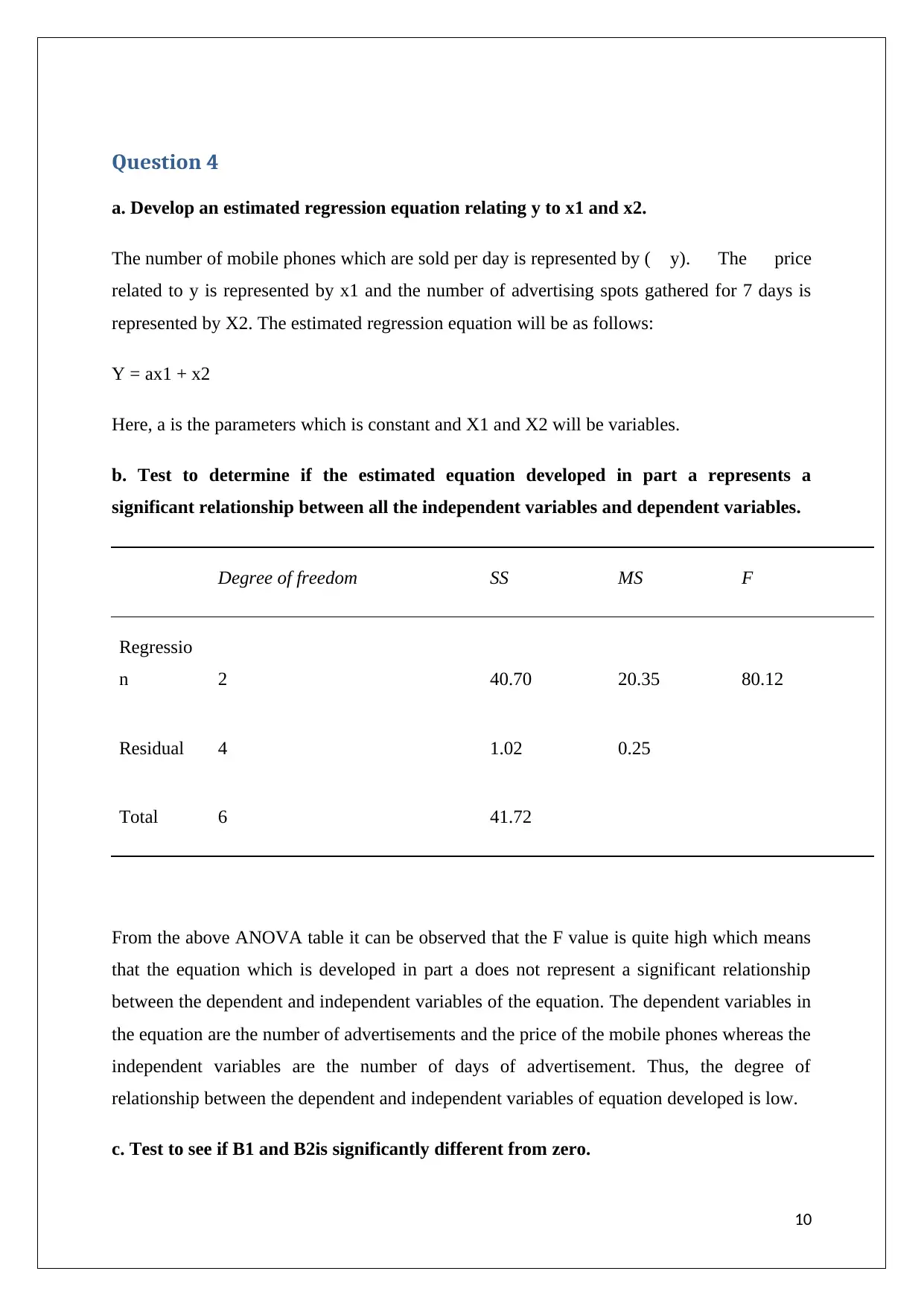
b. Test to determine if the estimated equation developed in part a represents a
significant relationship between all the independent variables and dependent variables.
Degree of freedom SS MS F
Regressio
n 2 40.70 20.35 80.12
Residual 4 1.02 0.25
Total 6 41.72
From the above ANOVA table it can be observed that the F value is quite high which means
that the equation which is developed in part a does not represent a significant relationship
between the dependent and independent variables of the equation. The dependent variables in
the equation are the number of advertisements and the price of the mobile phones whereas the
independent variables are the number of days of advertisement. Thus, the degree of
relationship between the dependent and independent variables of equation developed is low.
c. Test to see if B1 and B2is significantly different from zero.
10
a. Develop an estimated regression equation relating y to x1 and x2.
The number of mobile phones which are sold per day is represented by ( y). The price
related to y is represented by x1 and the number of advertising spots gathered for 7 days is
represented by X2. The estimated regression equation will be as follows:
Y = ax1 + x2
Here, a is the parameters which is constant and X1 and X2 will be variables.
b. Test to determine if the estimated equation developed in part a represents a
significant relationship between all the independent variables and dependent variables.
Degree of freedom SS MS F
Regressio
n 2 40.70 20.35 80.12
Residual 4 1.02 0.25
Total 6 41.72
From the above ANOVA table it can be observed that the F value is quite high which means
that the equation which is developed in part a does not represent a significant relationship
between the dependent and independent variables of the equation. The dependent variables in
the equation are the number of advertisements and the price of the mobile phones whereas the
independent variables are the number of days of advertisement. Thus, the degree of
relationship between the dependent and independent variables of equation developed is low.
c. Test to see if B1 and B2is significantly different from zero.
10
Paraphrase This Document
Need a fresh take? Get an instant paraphrase of this document with our AI Paraphraser
From the mean squares calculated using the sum of squares in the ANOVA table, it can be
observed that the difference between the mean square values of regression and residual is
very high. this means that the mean square values are different from zero to a large extent.
Thus, it can be said that b1 and b2 are significantly different from zero. The test is positive.
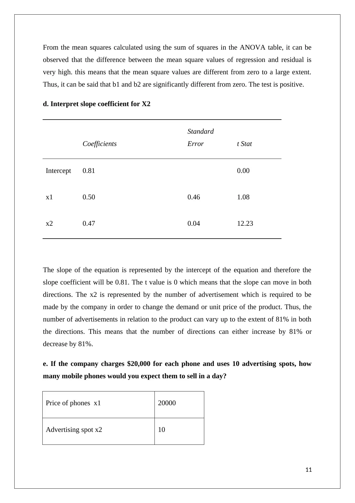
d. Interpret slope coefficient for X2
Coefficients
Standard
Error t Stat
Intercept 0.81 0.00
x1 0.50 0.46 1.08
x2 0.47 0.04 12.23
The slope of the equation is represented by the intercept of the equation and therefore the
slope coefficient will be 0.81. The t value is 0 which means that the slope can move in both
directions. The x2 is represented by the number of advertisement which is required to be
made by the company in order to change the demand or unit price of the product. Thus, the
number of advertisements in relation to the product can vary up to the extent of 81% in both
the directions. This means that the number of directions can either increase by 81% or
decrease by 81%.
e. If the company charges $20,000 for each phone and uses 10 advertising spots, how
many mobile phones would you expect them to sell in a day?
Price of phones x1 20000
Advertising spot x2 10
11
observed that the difference between the mean square values of regression and residual is
very high. this means that the mean square values are different from zero to a large extent.
Thus, it can be said that b1 and b2 are significantly different from zero. The test is positive.
d. Interpret slope coefficient for X2
Coefficients
Standard
Error t Stat
Intercept 0.81 0.00
x1 0.50 0.46 1.08
x2 0.47 0.04 12.23
The slope of the equation is represented by the intercept of the equation and therefore the
slope coefficient will be 0.81. The t value is 0 which means that the slope can move in both
directions. The x2 is represented by the number of advertisement which is required to be
made by the company in order to change the demand or unit price of the product. Thus, the
number of advertisements in relation to the product can vary up to the extent of 81% in both
the directions. This means that the number of directions can either increase by 81% or
decrease by 81%.
e. If the company charges $20,000 for each phone and uses 10 advertising spots, how
many mobile phones would you expect them to sell in a day?
Price of phones x1 20000
Advertising spot x2 10
11
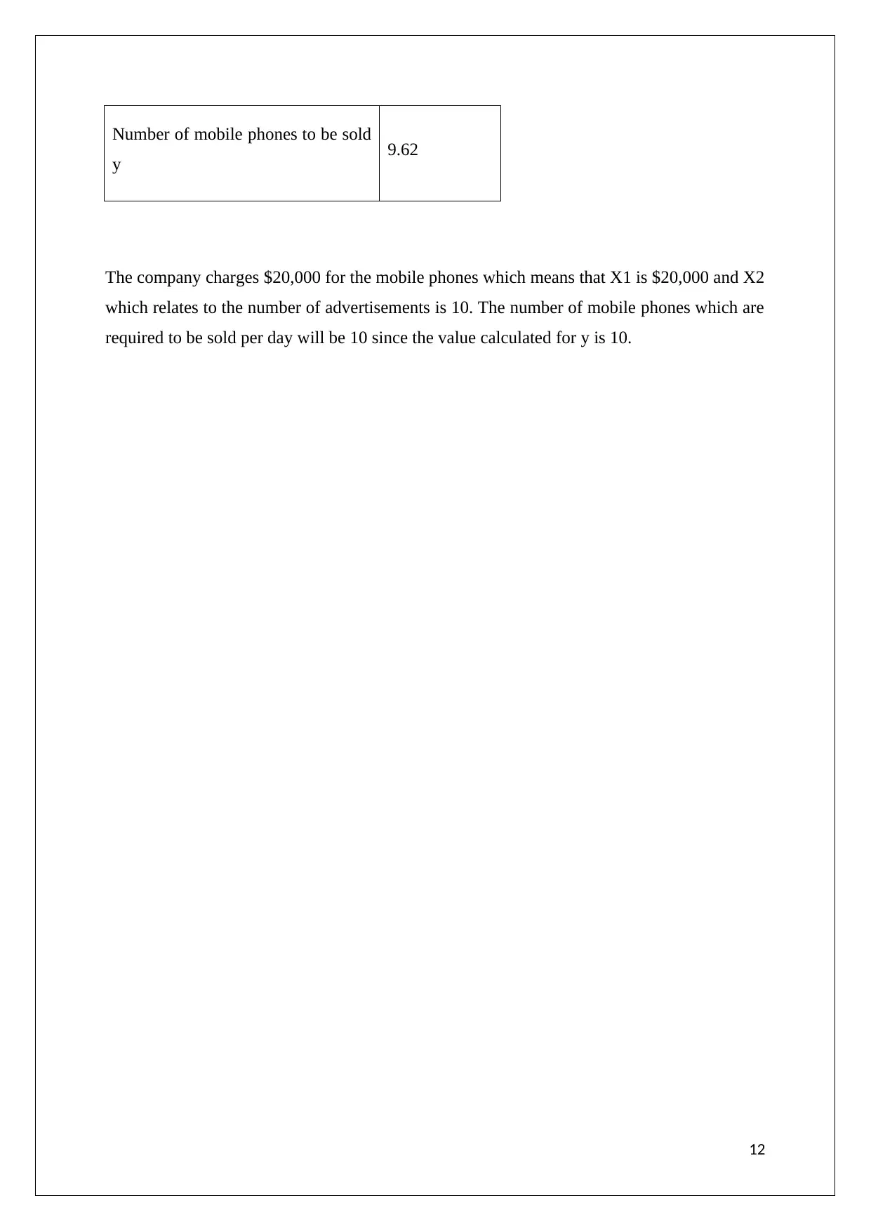
Number of mobile phones to be sold
y 9.62
The company charges $20,000 for the mobile phones which means that X1 is $20,000 and X2
which relates to the number of advertisements is 10. The number of mobile phones which are
required to be sold per day will be 10 since the value calculated for y is 10.
12
y 9.62
The company charges $20,000 for the mobile phones which means that X1 is $20,000 and X2
which relates to the number of advertisements is 10. The number of mobile phones which are
required to be sold per day will be 10 since the value calculated for y is 10.
12
⊘ This is a preview!⊘
Do you want full access?
Subscribe today to unlock all pages.
Trusted by 1+ million students worldwide
1 out of 13
Related Documents


Your All-in-One AI-Powered Toolkit for Academic Success.
+13062052269
info@desklib.com
Available 24*7 on WhatsApp / Email
![[object Object]](/_next/static/media/star-bottom.7253800d.svg)
Unlock your academic potential
Copyright © 2020–2026 A2Z Services. All Rights Reserved. Developed and managed by ZUCOL.