HI6007 Statistics: Analysis of Startup Costs and Sales Regression

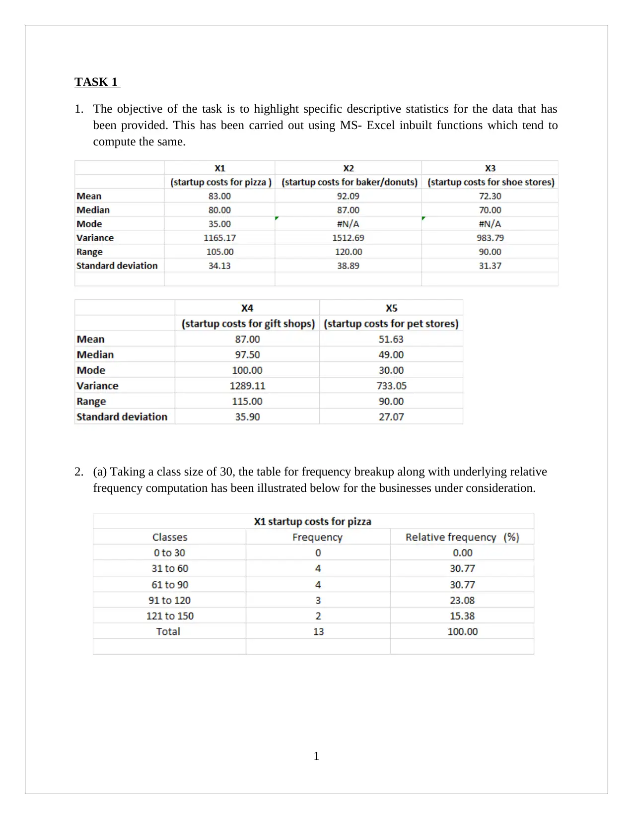
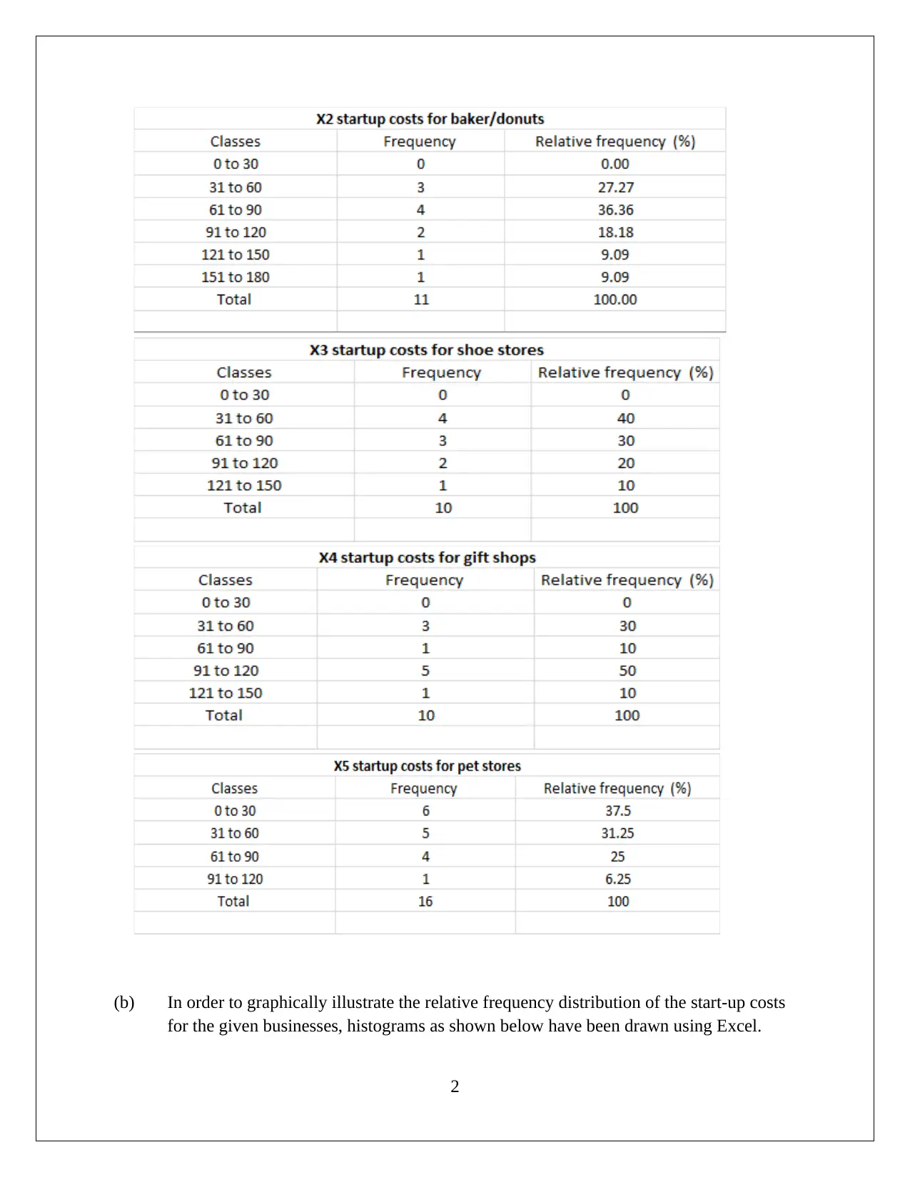
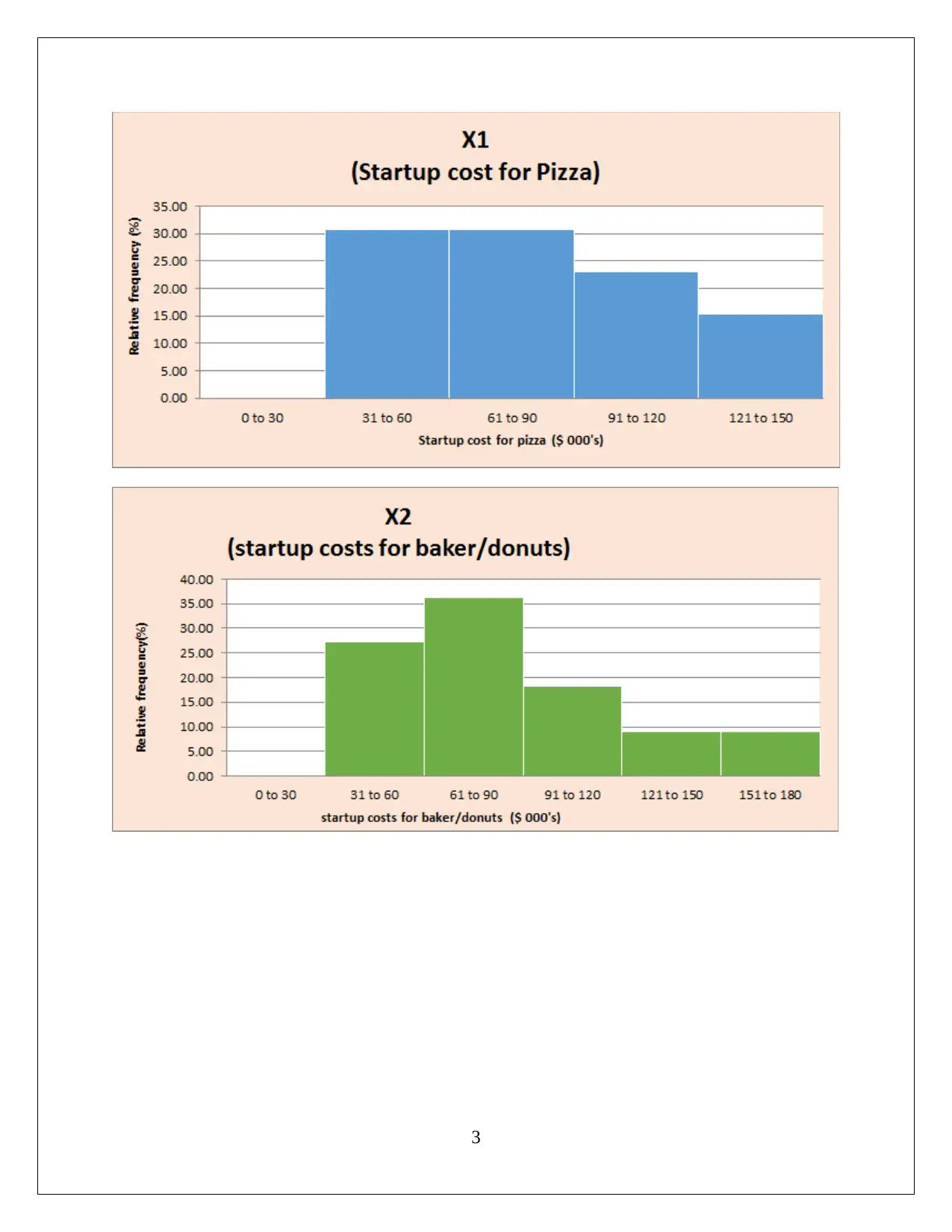
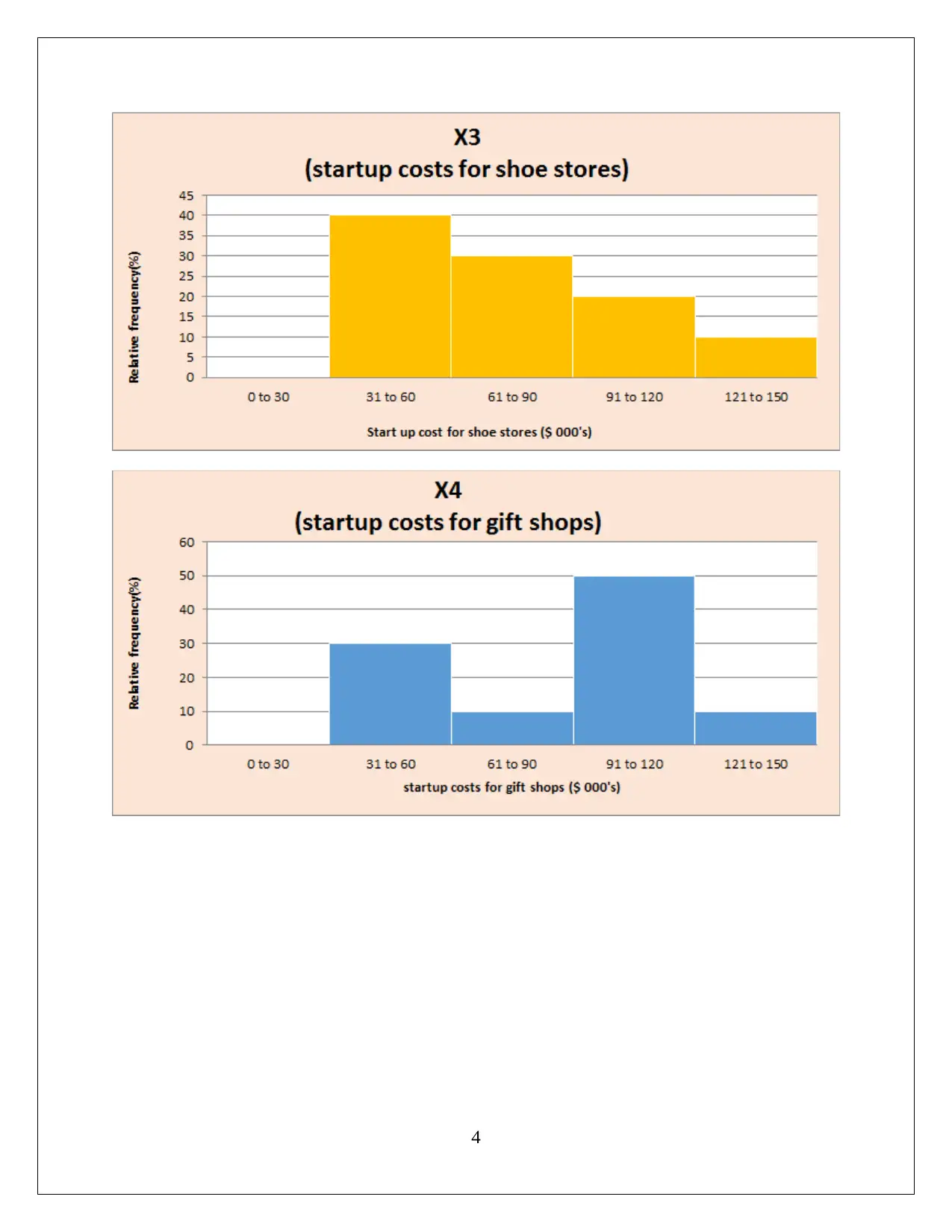
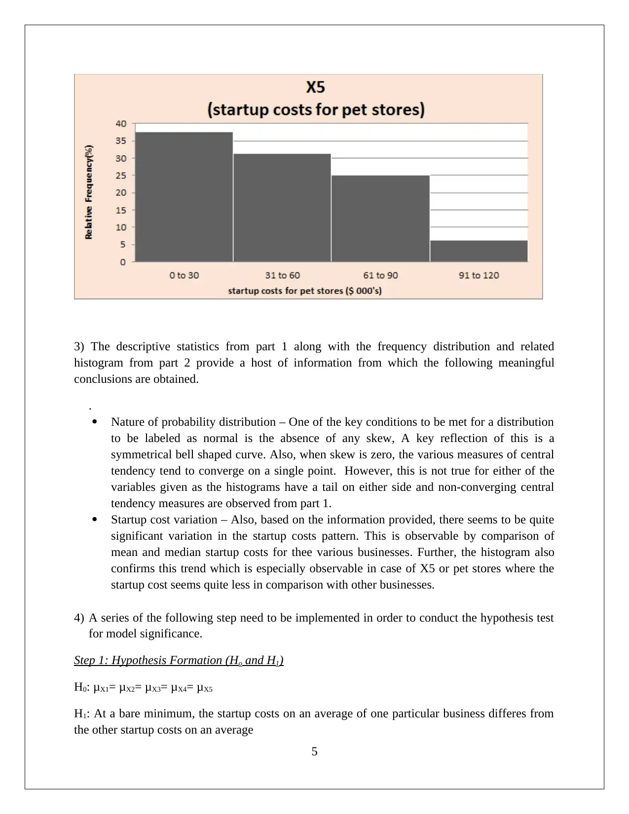
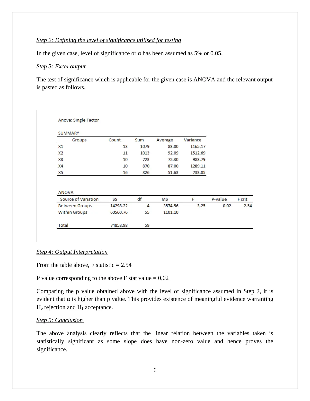
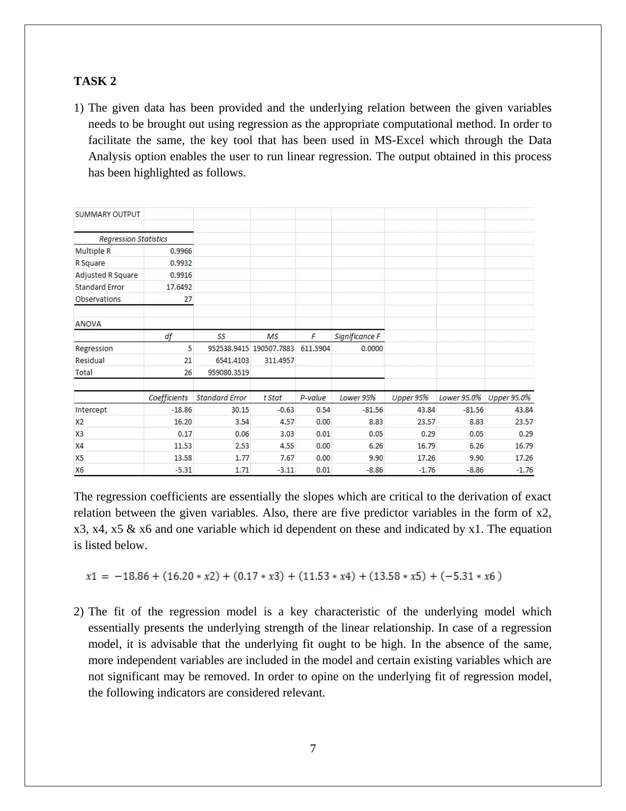
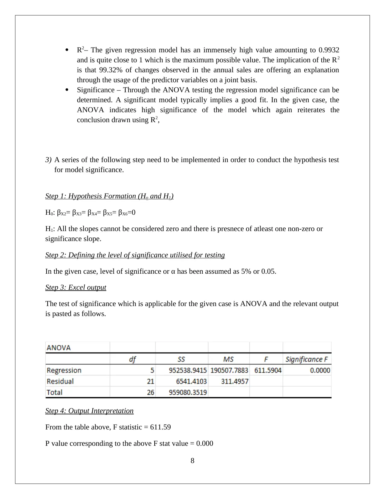
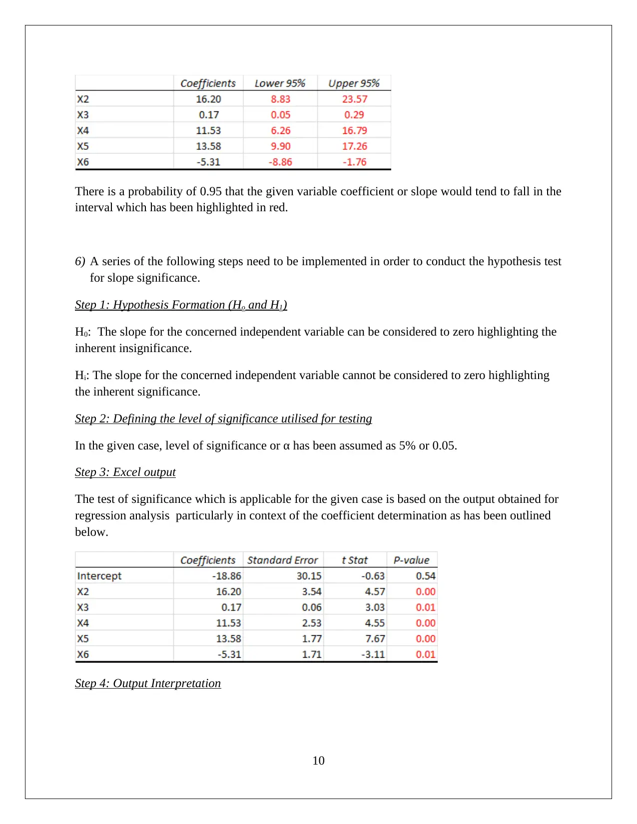
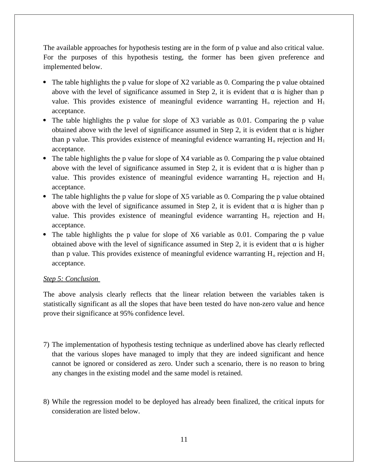
This assignment solution for HI6007 Statistics encompasses two key tasks. Task 1 focuses on descriptive statistics, including frequency distribution and histogram analysis of startup costs for various businesses. The solution highlights the nature of probability distribution, variation in startup costs, and conducts a hypothesis test using ANOVA to assess the significance of differences in startup costs. Task 2 delves into regression analysis, exploring the relationship between annual sales and predictor variables like franchise store area, inventory, advertising spending, customer coverage, and competing stores. The solution details the regression model's fit, interprets regression coefficients, and performs hypothesis tests for model and slope significance, ultimately concluding that the linear relationships are statistically significant. Finally, the solution provides a predictive model for annual sales based on given inputs.

HI6007 STATISTICS
Student id
[Pick the date]

TASK 1
1. The objective of the task is to highlight specific descriptive statistics for the data that has
been provided. This has been carried out using MS- Excel inbuilt functions which tend to
compute the same.
2. (a) Taking a class size of 30, the table for frequency breakup along with underlying relative
frequency computation has been illustrated below for the businesses under consideration.
1

(b) In order to graphically illustrate the relative frequency distribution of the start-up costs
for the given businesses, histograms as shown below have been drawn using Excel.
2

3

4

3) The descriptive statistics from part 1 along with the frequency distribution and related
histogram from part 2 provide a host of information from which the following meaningful
conclusions are obtained.
.
 Nature of probability distribution – One of the key conditions to be met for a distribution
to be labeled as normal is the absence of any skew, A key reflection of this is a
symmetrical bell shaped curve. Also, when skew is zero, the various measures of central
tendency tend to converge on a single point. However, this is not true for either of the
variables given as the histograms have a tail on either side and non-converging central
tendency measures are observed from part 1.
 Startup cost variation – Also, based on the information provided, there seems to be quite
significant variation in the startup costs pattern. This is observable by comparison of
mean and median startup costs for thee various businesses. Further, the histogram also
confirms this trend which is especially observable in case of X5 or pet stores where the
startup cost seems quite less in comparison with other businesses.
4) A series of the following step need to be implemented in order to conduct the hypothesis test
for model significance.
Step 1: Hypothesis Formation (Ho and H1)
H0: μX1= μX2= μX3= μX4= μX5
H1: At a bare minimum, the startup costs on an average of one particular business differes from
the other startup costs on an average
5

Step 2: Defining the level of significance utilised for testing
In the given case, level of significance or α has been assumed as 5% or 0.05.
Step 3: Excel output
The test of significance which is applicable for the given case is ANOVA and the relevant output
is pasted as follows.
Step 4: Output Interpretation
From the table above, F statistic = 2.54
P value corresponding to the above F stat value = 0.02
Comparing the p value obtained above with the level of significance assumed in Step 2, it is
evident that α is higher than p value. This provides existence of meaningful evidence warranting
Ho rejection and H1 acceptance.
Step 5: Conclusion
The above analysis clearly reflects that the linear relation between the variables taken is
statistically significant as some slope does have non-zero value and hence proves the
significance.
6

TASK 2
1) The given data has been provided and the underlying relation between the given variables
needs to be brought out using regression as the appropriate computational method. In order to
facilitate the same, the key tool that has been used in MS-Excel which through the Data
Analysis option enables the user to run linear regression. The output obtained in this process
has been highlighted as follows.
The regression coefficients are essentially the slopes which are critical to the derivation of exact
relation between the given variables. Also, there are five predictor variables in the form of x2,
x3, x4, x5 & x6 and one variable which id dependent on these and indicated by x1. The equation
is listed below.
2) The fit of the regression model is a key characteristic of the underlying model which
essentially presents the underlying strength of the linear relationship. In case of a regression
model, it is advisable that the underlying fit ought to be high. In the absence of the same,
more independent variables are included in the model and certain existing variables which are
not significant may be removed. In order to opine on the underlying fit of regression model,
the following indicators are considered relevant.
7

 R2– The given regression model has an immensely high value amounting to 0.9932
and is quite close to 1 which is the maximum possible value. The implication of the R2
is that 99.32% of changes observed in the annual sales are offering an explanation
through the usage of the predictor variables on a joint basis.
 Significance – Through the ANOVA testing the regression model significance can be
determined. A significant model typically implies a good fit. In the given case, the
ANOVA indicates high significance of the model which again reiterates the
conclusion drawn using R2,
3) A series of the following step need to be implemented in order to conduct the hypothesis test
for model significance.
Step 1: Hypothesis Formation (Ho and H1)
H0: βX2= βX3= βX4= βX5= βX6=0
H1: All the slopes cannot be considered zero and there is presnece of atleast one non-zero or
significance slope.
Step 2: Defining the level of significance utilised for testing
In the given case, level of significance or α has been assumed as 5% or 0.05.
Step 3: Excel output
The test of significance which is applicable for the given case is ANOVA and the relevant output
is pasted as follows.
Step 4: Output Interpretation
From the table above, F statistic = 611.59
P value corresponding to the above F stat value = 0.000
8

Comparing the p value obtained above with the level of significance assumed in Step 2, it is
evident that α is higher than p value. This provides existence of meaningful evidence warranting
Ho rejection and H1 acceptance.
Step 5: Conclusion
The above analysis clearly reflects that the linear relation between the variables taken is
statistically significant as some slope does have non-zero value and hence proves the
significance.
4) The slope interpretation essentially involves analyzing the respective coefficients considering
their sign as well as magnitude. The presence of a + sign denotes that the change in both
dependent and independent variable would be in the same direction. However, the presence of
a – sign denotes that the change in both dependent and independent variable would be in the
opposite direction. Further, the quantum of change that is expected to be seen in the
dependent variable would depend on the magnitude of the slope along with the respective
change in the independent variable. Considering the general norms highlighted, the slope
interpretation is offered as follows.
 X2 (Value is 16.20) – The given slope reflects that any change in the franchise store area
by 1 unit (i.e. 1 sq. ft) would produce an alteration in annual sales by $ 16.20 and that too
in the same direction.
 X3 (Value is 0.17) - The given slope reflects that any change in the franchise store
inventory by 1 unit (i.e.$1) would produce an alteration in annual sales by $ 0.17 and that
too in the same direction.
 X4 (Value is 11.53) - The given slope reflects that any change in the franchise store
advertising spending by 1 unit (i.e.$1) would produce an alteration in annual sales by $
11.53 and that too in the same direction.
 X5 (Value is 13.58) - The given slope reflects that any change in the franchise store
customer coverage by 1 unit (i.e. one family) would produce an alteration in annual sales
by $ 13,58 and that too in the same direction..
 X6 (Value is -5.31) - The given slope reflects that any change in the franchise store
competing stores by one would produce an alteration in annual sales by $ 5,310 and that
too in the opposite direction.
5) The summary of the slope coefficients in relation to their defining the 95% confidence
interval is presented in the tabular manner as follows.
.
9

There is a probability of 0.95 that the given variable coefficient or slope would tend to fall in the
interval which has been highlighted in red.
6) A series of the following steps need to be implemented in order to conduct the hypothesis test
for slope significance.
Step 1: Hypothesis Formation (Ho and H1)
H0: The slope for the concerned independent variable can be considered to zero highlighting the
inherent insignificance.
Hi: The slope for the concerned independent variable cannot be considered to zero highlighting
the inherent significance.
Step 2: Defining the level of significance utilised for testing
In the given case, level of significance or α has been assumed as 5% or 0.05.
Step 3: Excel output
The test of significance which is applicable for the given case is based on the output obtained for
regression analysis particularly in context of the coefficient determination as has been outlined
below.
Step 4: Output Interpretation
10

The available approaches for hypothesis testing are in the form of p value and also critical value.
For the purposes of this hypothesis testing, the former has been given preference and
implemented below.
 The table highlights the p value for slope of X2 variable as 0. Comparing the p value obtained
above with the level of significance assumed in Step 2, it is evident that α is higher than p
value. This provides existence of meaningful evidence warranting Ho rejection and H1
acceptance.
 The table highlights the p value for slope of X3 variable as 0.01. Comparing the p value
obtained above with the level of significance assumed in Step 2, it is evident that α is higher
than p value. This provides existence of meaningful evidence warranting Ho rejection and H1
acceptance.
 The table highlights the p value for slope of X4 variable as 0. Comparing the p value obtained
above with the level of significance assumed in Step 2, it is evident that α is higher than p
value. This provides existence of meaningful evidence warranting Ho rejection and H1
acceptance.
 The table highlights the p value for slope of X5 variable as 0. Comparing the p value obtained
above with the level of significance assumed in Step 2, it is evident that α is higher than p
value. This provides existence of meaningful evidence warranting Ho rejection and H1
acceptance.
 The table highlights the p value for slope of X6 variable as 0.01. Comparing the p value
obtained above with the level of significance assumed in Step 2, it is evident that α is higher
than p value. This provides existence of meaningful evidence warranting Ho rejection and H1
acceptance.
Step 5: Conclusion
The above analysis clearly reflects that the linear relation between the variables taken is
statistically significant as all the slopes that have been tested do have non-zero value and hence
prove their significance at 95% confidence level.
7) The implementation of hypothesis testing technique as underlined above has clearly reflected
that the various slopes have managed to imply that they are indeed significant and hence
cannot be ignored or considered as zero. Under such a scenario, there is no reason to bring
any changes in the existing model and the same model is retained.
8) While the regression model to be deployed has already been finalized, the critical inputs for
consideration are listed below.
11